Introduction

Let’s begin with the simplest question: what, exactly, is a join? If you remember the SQL project, you’ll remember writing things like R INNER JOIN S ON R.name = S.name and other similar statements. What that actually meant is that you take two relations, R and S, and create one new relation out of their matches on the join condition – that is, for each record \(r_i\) in R, find all records \(s_j\) in S that match the join condition we have specified and write \(<r_i, s_j>\) as a new row in the output (all the fields of r followed by all the fields of s). The SQL lecture slides are a great resource for more clarifications on what joins actually are.¹ Before we get into the different join algorithms, we need to discuss what happens when the new joined relation consisting of \(<r_i, s_j>\) is formed. Whenever we compute the cost of a join, we will ignore the cost of writing the joined relation to disk. This is because we are assuming that the output of the join will be consumed by another operator involved later on in the execution of the SQL query. Often times this operator can directly consume the joined records from memory so we don’t need to write the joined table to disk. Don’t worry if this sounds confusing right now; we will revisit it in the Query Optimization module, but the important thing to remember for now is that the final write cost is not included in our join cost models!

Simple Nested Loop Join

Let’s start with the simplest strategy possible. Let’s say we have a buffer of B pages, and we wish to join two tables, R and S, on the join condition \(\theta\). Starting with the most naïve strategy, we can take each record in R, search for all its matches in S, and then we yield each match. This is called simple nested loop join (SNLJ). You can think of it as two nested for loops: \

for each record \(r_i\) in R:

    for each record \(s_j\) in S:

        if \(\theta\)(\(r_i\),\(s_j\)):

            yield <\(r_i\), \(s_j\)>

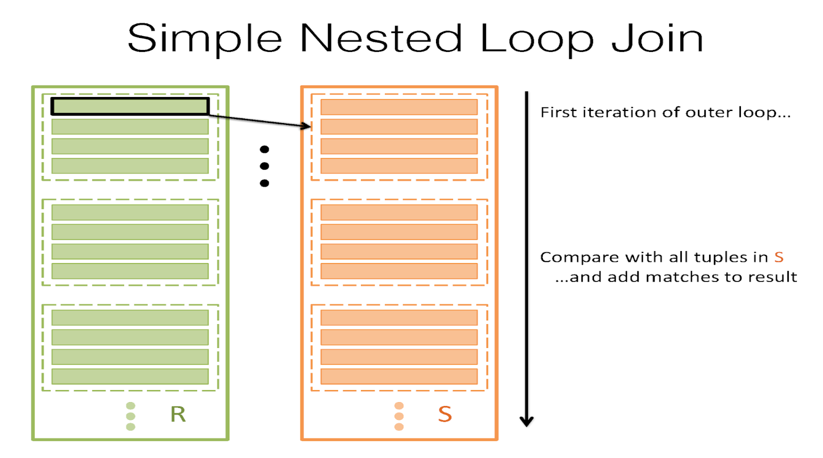
This would be a great thing to do, but the theme of the class is really centered around optimization and minimizing I/Os. For that, this is a pretty poor scheme, because we take each record in R and read in every single page in S searching for a match. The I/O cost of this would then be \([R]+|R|[S]\), where [R] is the number of pages in R and |R| is the number of records in R. And while we might be able to optimize things a slight amount by switching the order of R and S in the for loop, this really isn’t a very good strategy. Note: SNLJ does not incur |R| I/Os to read every record in R. It will cost [R] I/Os because it’s really doing something more like “for each page \(p_r\) in R: for each record \(r\) in \(p_r\): for each page \(p_s\) in S: for each record \(s\) in \(p_s\): join” since we can’t read less than a page at a time.

Page Nested Loop Join

It’s clear that we don’t want to read in every single page of S for each record of R, so what can we do better? What if we read in every single page in S for every single page of R instead? That is, for a page of R, take all the records and match them against each record in S, and do this for every page of R. That’s called page nested loop join (PNLJ). Here’s the pseudocode for it:

for each page \(p_r\) in R:

    for each page \(p_s\) in S:

        for each record \(r_i\) in \(p_r\):

            for each record \(s_j\) in \(p_s\):

                if \(\theta\)(\(r_i\), \(s_j\)):

                    yield <\(r_i\), \(s_j\)>

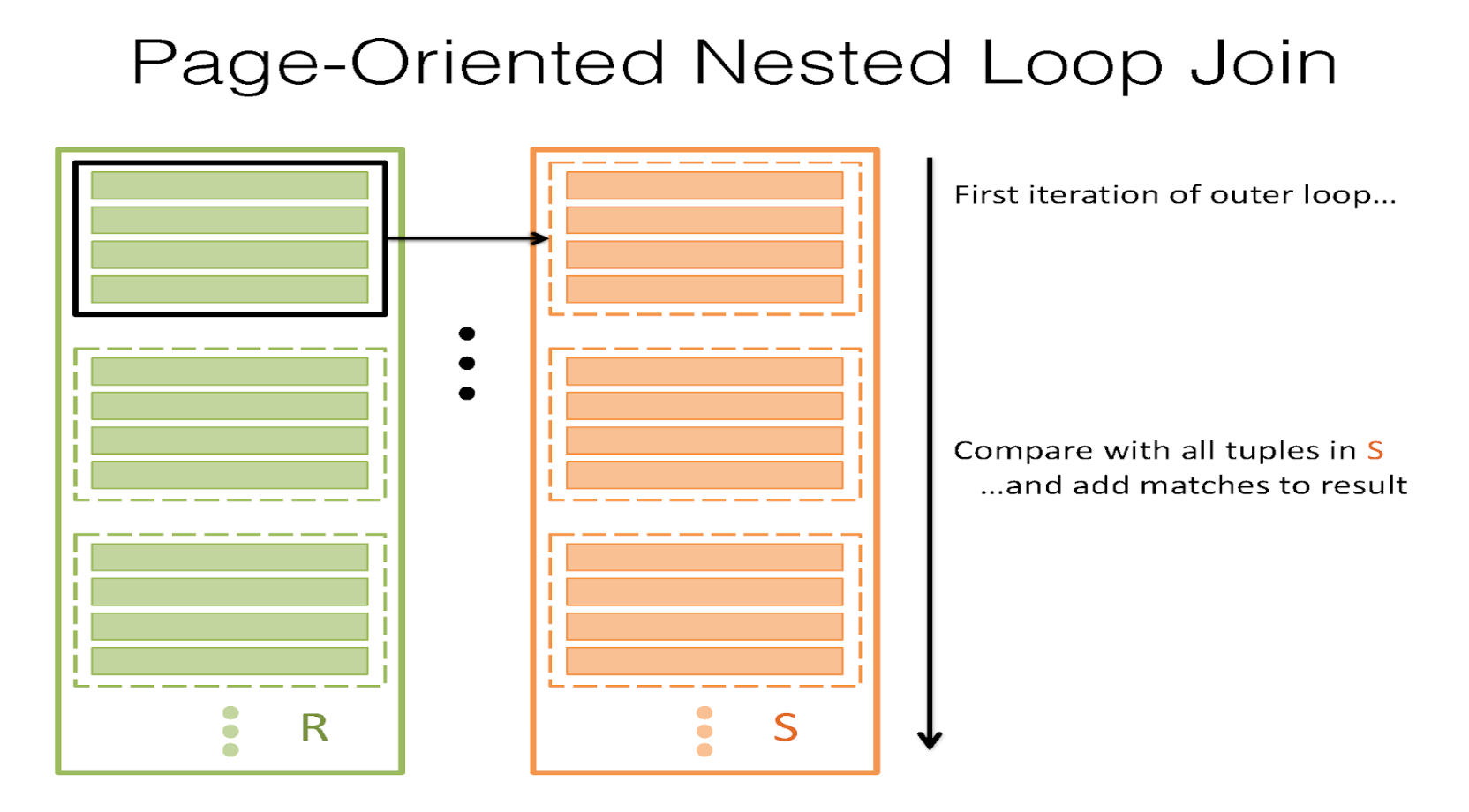
The I/O cost of this is somewhat better. It’s \([R]+[R]∗[S]\) – this can be optimized by keeping the smaller relation between R and S as the outer one (keep this in mind when asked to find the lowest cost for performing the join).

Block Nested Loop Join

Page Nested Loop Join is a lot better! The only problem is that we’re still not fully utilizing our buffer as powerfully as we can. We have B buffer pages, but our algorithm only uses 3 – one for R, one for S, and one for the output buffer. Remember that the fewer times we read in S, the better – so if we can reserve B-2 pages for R instead and match S against every record in each "chunk", we could cut down our I/O cost drastically! In this join, \(B-2\) pages are for R, 1 page is for S, and 1 page is the output buffer for the join. This is called Chunk Nested Loop Join (or Block Nested Loop Join). The key idea here is that we want to utilize our buffer to help us reduce the I/O cost, and so we can reserve as many pages as possible for a chunk of R – because we only read in each page of S once per chunk, larger chunks imply fewer I/Os. For each chunk of R, match all the records in S against all the records in the chunk.

for each block of B-2 pages \(B_r\) in R:

    for each page \(p_s\) in S:

        for each record \(r_i\) in \(B_r\):

            for each record \(s_j\) in \(p_s\):

                if \(\theta\)(\(r_i\),\(s_j\)):

                    yield <\(r_i\), \(s_j\)>

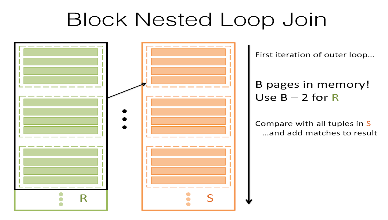
Then, the I/O cost of this can be written as \([R]+\lceil{\frac{[R]}{B-2}}\rceil[S]\). This is a lot better! Now, we’re taking advantage of our B buffer pages to reduce the number of times we have to read in S. See Project 3 Part 1 Task 1 for a dynamic visualization of BNLJ in action!

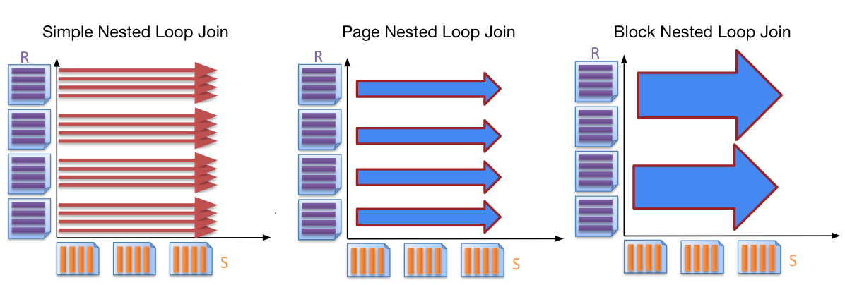
Visual Comparison of Loop Joins

Index Nested Loop Join

There are times, however, when Block Nested Loop Join isn’t the best thing to do. Sometimes, if we have an index on S that is on the appropriate field (i.e. the field we are joining on), it can be very fast to look up matches of \(r_i\) in S. This is called index nested loop join, and the pseudocode goes like this:

for each record \(r_i\) in R:

    for each record \(s_j\) in S where \(\theta\)(\(r_i\),\(s_j\)) == \(true\):

        yield <\(r_i\), \(s_j\)>

The I/O cost is \([R] + |R| *\)(cost to look up matching records in S). The cost to look up matching records in S will differ based on the type of index (alternative 1, 2, 3 and unclustered vs. clustered). If it is a B+ tree, we will search starting at the root and count how many I/Os it will take to get to a corresponding record. See the Clustering and Counting I/O’s sections of the B+ tree course notes.

Hash Join

Notice that in this entire sequence, we’re really trying to look for matching records. Hash tables are really nice for looking up matches, though; even if we don’t have an index, we can construct a hash table that is B-2 pages² big on the records of R, fit it into memory, and then read in each record of S and look it up in R’s hash table to see if we can find any matches on it. This is called Naive Hash Join. Its cost is \([R] + [S]\) I/Os. That’s actually the best one we’ve done yet. It’s efficient, cheap, and simple. There’s a problem with this, however; this relies on R being able to fit entirely into memory (specifically, having R being \(\leq B-2\) pages big). And that’s often just not going to be possible. To fix this, we repeatedly hash R and S into B-1 buffers so that we can get partitions that are \(\leq B-2\) pages big, enabling us to fit them into memory and perform a Naive Hash Join. More specifically, consider each pair of corresponding partitions R\(_i\) and S\(_i\) (i.e. partition i of R and partition i of S). If R\(_i\) and S\(_i\) are both \(>\) B-2 pages big, hash both partitions into smaller ones. Else, if either R\(_i\) or S\(_i\) \(\leq\) B-2 pages, stop partitioning and load the smaller partition into memory to build an in-memory hash table and perform a Naive Hash Join with the larger partition in the pair. This procedure is called Grace Hash Join, and the I/O cost of this is: the cost of hashing plus the cost of Naive Hash Join on the subsections. The cost of hashing can change based on how many times we need to repeatedly hash on how many partitions. The cost of hashing a partition P includes the I/O’s we need to read all the pages in P and the I/O’s we need to write all the resulting partitions after hashing partition P. The Naive Hash Join portion cost per partition pair is the cost of reading in each page in both partitions after you have finished. Grace Hash is great, but it’s really sensitive to key skew, so you want to be careful when using this algorithm. Key skew is when we try to hash but many of the keys go into the same bucket. Key skew happens when many of the records have the same key. For example, if we’re hashing on the column which only has "yes" as values, then we can keep hashing but they will all end up in the same bucket no matter which hash function we use.

Sort-Merge Join

There’s also times when it helps for us to sort R and S first, especially if we want our joined table to be sorted on some specific column. In those cases, what we do is first sort R and S. Then:

(1) we begin at the start of R and S and advance one or the other until we get to a match (if \(r_i<s_j\), advance R; else if \(r_i>s_j\), advance S – the idea is to advance the lesser of the two until we get to a match).

(2) Now, let’s assume we’ve gotten to a match. Let’s say this pair is \(r_i,s_j\). We mark this spot in S as \(marked(S)\) and check each subsequent record in S (\(s_j\),\(s_{j+1}\),\(s_{j+2}\), etc) until we find something that is not a match (i.e. read in all records in S that match to \(r_i\)).

(3) Now, go to the next record in R and go back to the marked spot in S and begin again at step 1 (except instead of beginning at the start of R and the start of S, do it at the indices we just indicated) – the idea is that because R and S are sorted, any match for any future record of R cannot be before the marked spot in S, because this record \(r_{i+1} \geq r_i\) – if a match for \(r_i\) did not exist before \(marked(S)\), a match for \(r_{i+1}\) cannot possibly be before \(marked(S)\) either! So we scroll from the marked spot in S until we find a match for \(r_{i+1}\).

This is called Sort-Merge Join and the average I/O cost is: cost to sort R + cost to sort S + (\([R] + [S]\)) (though it is important to note that this is not the worst case!). In the worst case, if each record of R matches every record of S, the last term becomes \(|R|*[S]\). The worst case cost is then: cost to sort R + cost to sort S + \(([R] + |R| * [S])\). That generally doesn’t happen, though).

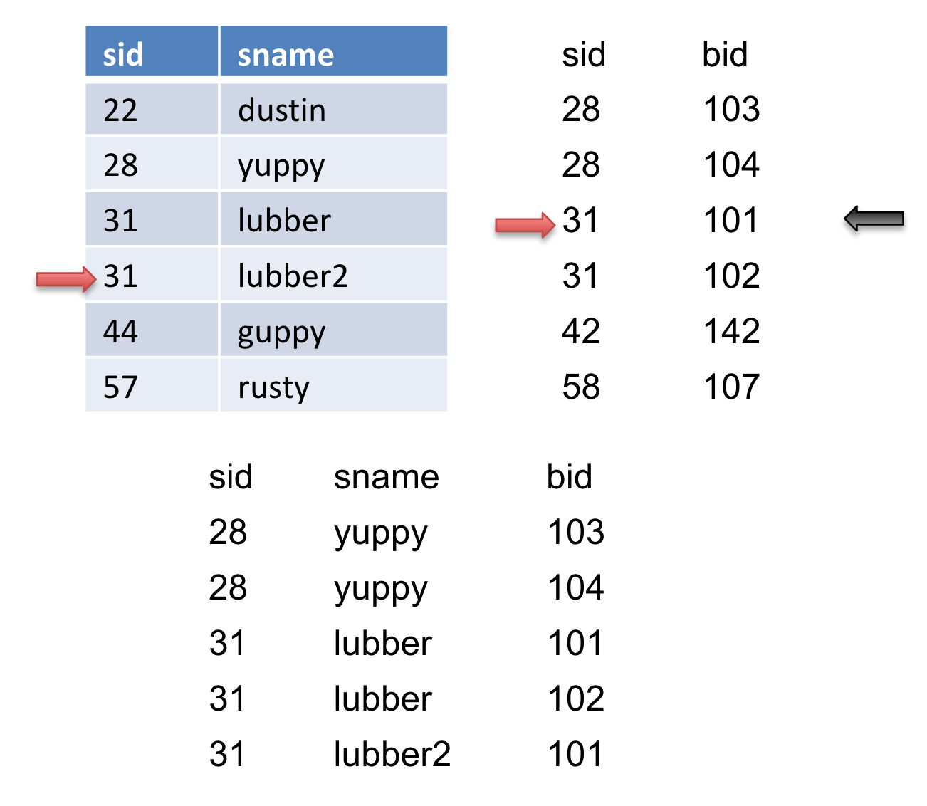
Let’s take a look at an example. Let the table on the left be \(R\) and the table on the right be \(S\).

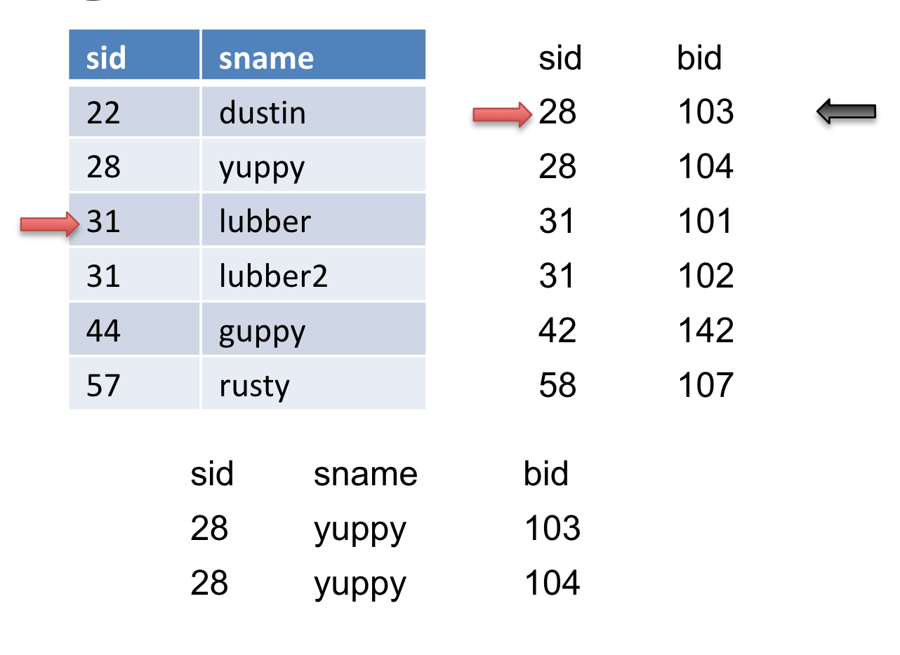
We will advance the pointer (the red arrow) on \(S\) because \(28<31\) until \(S\) gets to sid of \(31\). Then we will mark this record (the black arrow). In addition, we will output this match.

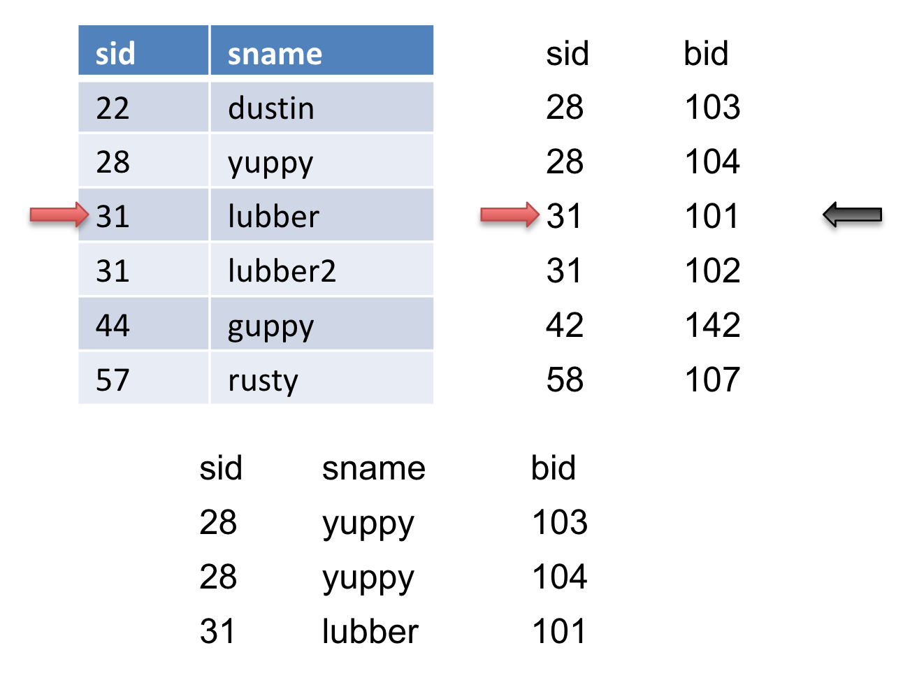
Then we will advance the pointer on \(S\) again and we get another match and output it.

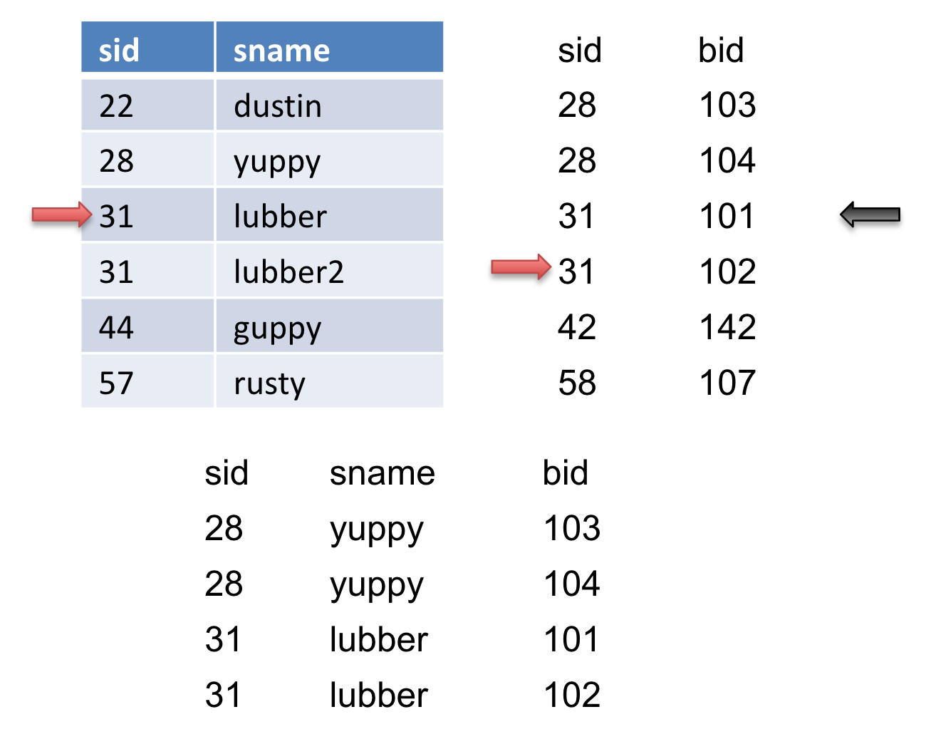
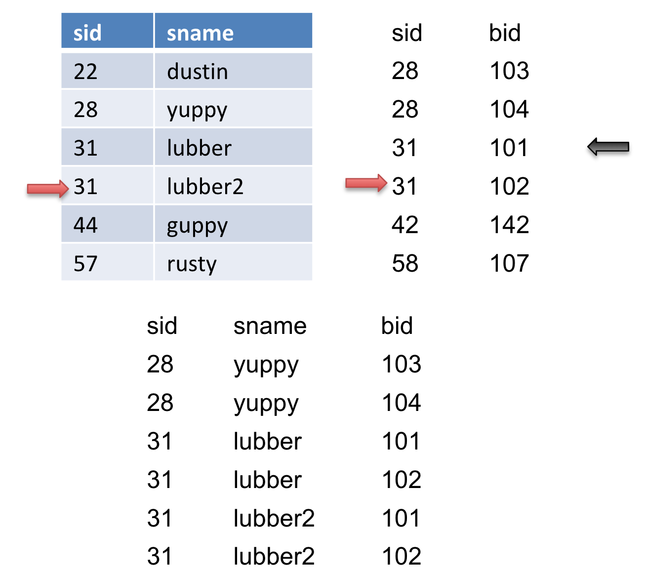
We advance the pointer on \(S\) again, but we do not get a match. We then reset \(S\) to where we marked (the black arrow) and then advance \(R\). When we advance \(R\), we get another match so we output it.

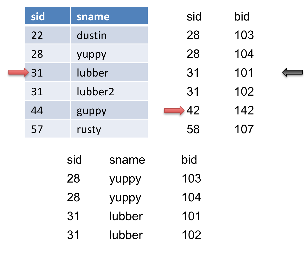
We then advance \(S\), we get another match so we output it.

do {
    if (!mark) {
        while (r < s) { advance r }
        while (r > s) { advance s }
        // mark start of “block” of S
        mark = s
     }
    if (r == s) {
        result = <r, s>
        advance s
        yield result
    }
    else {
        reset s to mark
        advance r
        mark = NULL
    }
}

An Important Refinement

An important refinement: You can combine the last sorting phase with the merging phase, provided you have enough room in memory to allocate a page for each run of [R] and for each run of [S]. The final merge pass is where you allocate a page for each run of R and each run of S. In this process, you save \(2*([R] + [S])\) I/Os To perform the optimization, we must

(1) sort [R] and [S] (individually, using the full buffer pool for each of them) until you have them both "almost-sorted"; that is, for each table T in {R, S}, keep merging runs of T until you get to the penultimate step, where one more sorting pass would result in a sorted table T.

(2) See how many runs of [R] and how many runs of [S] are left; sum them up. Allocate one page in memory for each run. If you have enough input buffers left to accommodate this (i.e. if runs(R) + runs(S) \(\leq B-1\)), then you may use the optimization and you could then save \(2*([R] + [S])\) I/Os.

(3) If you could not do the optimization described in the previous step, it means that runs(R) + runs(S) \(\geq\) B. In the ideal case, the optimization allows us to avoid doing an extra read of both R and S, but this is not possible here, as we don’t have an available buffer for each run of R and S.

However, we’re not out of options yet! If we can’t avoid extra reads for both \(R\) and \(S\), perhaps we can avoid an extra read for at least one of them. Let’s assume that the outer relation R is the larger relation in this join. Because we are trying to minimize I/Os, we would like to avoid the extra read for the larger table \(R\). Could it help us to maybe completely sort just the smaller table \(S\) and use that in an optimization? It turns out that we can! If we completely sort \(S\), there is, by definition, now only one sorted run for that table, and this would mean that we only need to allocate one page in our buffer for it. So, if runs(\(R\)) + 1 \(\leq B - 1\), then we can allocate one buffer page for \(S\) and for each run of \(R\). Then, we can perform the SMJ optimization. Here, we have avoided the final sorting pass for \(R\) by combining it with the join phase. So we have saved \(2*[R]\) pages. Sometimes, though, even this is not enough – if runs(\(R\)) = B-1, then we don’t have a spare buffer page for \(S\). In this case, we’d like to still reduce as many I/Os as possible, so maybe perform the procedure described in the previous paragraph, but for the smaller table. That is, if runs(\(S\)) + 1 \(\leq B-1\), then sort \(R\), reducing the number of sorted runs for it to 1 by definition, and then allocate one buffer page for \(R\) and one for each run of \(S\). Then, perform the optimization – this will enable us to avoid the final sorting pass for \(S\) by combining it with the join phase, saving us \(2*[S]\) I/Os. When determining the cost of SMJ, any optimizations that can be applied should be used. If none of those conditions are met, though, we just won’t be able to optimize sort-merge join. And that’s alright. Sometimes, we just have to bite the bullet and accept that we can’t always cut corners.

Practice Questions

1. Sanity check - determine whether each of the following statements is true or false.

   a. Block Nested Loops join will always perform at least as well as Page Nested Loops Join when it comes to minimizing I/Os.

   b. Grace hash join is usually the best algorithm for joins in which the join condition includes an inequality (i.e. col1 \(<\) col2).

2. We have a table R with 100 pages and S with 50 pages and a buffer of size 12. What is the cost of a page nested loop join of R and S?

3. Given the same tables, R and S, from the previous question, we now also have an index on table R on the column a. If we are joining R.b == S.b, can we use index nested loop join?

4. Given the same tables, R and S, we want to join R and S on R.b == S.b. What is the cost of an index nested loop join of R and S?

   Assume the following for this problem only:

   • \(\rho_R = 10\) (meaning there are 10 records per page within R)

   • \(\rho_S = 30\) (meaning there are 30 records per page within S)

   • For every tuple in R, there are 5 tuples in S that satisfy the join condition and for every tuple in S, there are 20 tuples in R that satisfy the join condition.

   • There is an Alt. 3 clustered index on R.b of height 3.

   • There is an Alt. 3 unclustered index on S.b of height 2.

   • There are only 3 buffer pages available.

5. Then we realize that R is already sorted on column b so we decide to attempt a sort merge join. What is the cost of the sort merge join of R and S?

6. Lastly, we try Grace Hash Join on the two tables. Assume that the hash uniformly distributes the data for both tables. What is the cost of Grace Hash Join of R and S?

Solutions

1. True, False

   a. True - Block Nested Loops Join turns into PNLJ when B=3. Otherwise the cost model is strictly less: \([R] + [R]*[S]\) vs \([R] + [R/(B-2)] * [S]\)

   b. False - A hash join requires an Equijoin which cannot happen when an inequality is involved.

2. It does not matter the size of the buffer because we are doing a page nested loop join which only requires 3 buffer pages (one for R, one for S, and one for output). We will consider both join orders: \([R] + [R][S] = 100 + 100 * 50 = 5100\) \([S] + [S][R] = 50 + 50 * 100 = 5050\) The second join order is optimal and the number of I/O’s is 5050.

3. The answer is no, we cannot use index nested loop join because the index is on the column a which is not going to help us since we are joining on B.

4. Recall the generic formula for an index nested loop join: \([R] + |R| *\)(cost to look up matching records in S).

   Let’s first compute the cost of R join S.

   We know that \(|R| = [R] * \rho_R = 100 * 10\) = 1000 records.
   The cost to lookup a record in the unclustered index on S.b of height 2 will cost: 3 I/Os to read the root to the leaf node and 1 more I/O to read the actual tuple from the data page. Since we have 5 tuples in S that match every tuple in R and the S.b index is unclustered the cost to find the matching records in S will be 3 + 5 = 8 I/Os. Also, because the index is Alt. 3, we know all matching (key, rid) entries will be stored on the same leaf node, so we only need to read in 1 leaf node.

   Therefore, R INLJ S costs \(100 + 1000*8\) = 8100 I/Os.

   We now compute the cost of S join R.

   We know that \(|S| = [S] * \rho_S = 50 * 30\) = 1500 records.
   The cost to lookup a record in the clustered index on R.b of height 3 will cost: 4 I/Os to read the root to the leaf node and 1 I/O for every page of matching tuples. Since there are 20 tuples in R that satisfy the join condition for each tuple in S and \(\rho_R = 10\), each index lookup will result in 2 pages of matching tuples, which costs 2 I/Os to read. Thus, the cost to find the matching records in R will be 4 + 2 = 6 I/Os. Also, because the index is Alt. 3, we know all matching (key, rid) entries will be stored on the same leaf node, so we only need to read in 1 leaf node.

   Therefore, S INLJ R costs \(50 + 1500*6\) = 9050 I/Os.

   The first join order is optimal so the cost of the INLJ is 8100 I/Os.

5. Since R is already sorted, we just have to sort S which will take 2 passes because \(B=12\). The first pass creates \(\lceil{\frac{50}{11}}\rceil\) runs, which is 5 runs. And then we merge the tables together using one more pass, the merge pass. The total cost is therefore \(2 * 2 * [S] + [R] + [S] = 4 * 50 + 100 + 50 = 350\)

6. First, we need to partition both tables into partitions of size \(B-2\) or smaller.

   For R: \(ceil(100 / 11) = 10\) pages per partition after first pass

   For S: \(ceil(50/11) = 5\) pages per partition after first pass

   As we see from above, each table only needs one pass to be partitioned. We will have \(100\) I/O’s for reading in table R and then \(11*10=110\) I/O’s to write the partitions of table R back to disk. Similar calculations are done for table S. We will have \(50\) I/O’s for reading in table S and \(11*5=55\) I/O’s to write the partitions of S back to disk.

   Then we join the corresponding partitions together. To do this, we will have to read in \(11\) partitions of table R and \(11\) partitions of table S. This gives us \(11 * 10 = 110\) I/O’s for reading partitions of table R and \(11*5 = 55\) I/O’s for reading partitions of table S.

   Therefore, our total I/O cost will be \(100\) (read R)\(+ 110\) (write R after partition)\(+ 50\) (read S)\(+ 55\) (write S after partition)\(+ 110 + 55 = 480\)

1. notation aside: [T] is the number of pages in table T, \(\rho_{T}\) is the number of records on each page of T, and |T| is the total number of records in table T. In other words, |T| = [T] \(\times \ \rho_{T}\). This is really essential to understand the following explanations. ↩

2. We need one page for the current page in S and one page to store output records. The other B-2 pages can be used for the hash table. ↩