Introduction
Most of the semester has focused on the properties and implementation of relational database management systems, but here we will take a detour to explore a relatively new1 class of database that has come to be called NoSQL. NoSQL databases deviate from the set of database design principles that we have studied in order to achieve the high scale and elasticity needed for modern “Web 2.0” applications. In this document we will explore the motivation and history of NoSQL databases, review the design and properties of several types of NoSQL databases, compare the NoSQL data model with the relational data model, and conclude with a description of MongoDB, a popular and representative NoSQL database.
Motivation and History
OLTP and OLAP
In order to understand the emergence and properties of NoSQL, we must first describe two broad classes of workloads that can be subjected to a database.
Online Transaction Processing (OLTP) is a class of workloads characterized by high numbers of transactions executed by large numbers of users. This kind of workload is common to “frontend” applications such as social networks and online stores. Queries are typically simple lookups (e.g., “find user by ID”, “get items in shopping cart”) and rarely include joins. OLTP workloads also involve high numbers of updates (e.g., “post tweet”, “add item to shopping cart”). Because of the need for consistency in these business-critical workloads, the queries, inserts and updates are performed as transactions.
Online Analytical Processing is a class of read-only workloads characterized by queries that typically touch a large amount of data. OLAP queries typically involve large numbers of joins and aggregations in order to support decision making (e.g., “sum revenues by store, region, clerk, product, date”).
In many cases, OLTP and OLAP workloads are served by separate databases. Data must be migrated from OLTP systems to OLAP systems every so often via a process called extract-transform-load (ETL).
| Property | OLTP | OLAP |
|---|---|---|
| Main read pattern | Small number of records per query, fetched by key | Aggregate over large number of records |
| Main write pattern | Random-access, low-latency writes from user input | Bulk import or event stream |
| Primarily used by | End user/customer, via web application | Internal analysis, for decision support |
| What data represents | Latest state of data (current point in time) | History of events that happend over time |
| Dataset size | Gigabytes to terabytes | Terabytes to petabytes |
Table from Designing Data-Intensive Applications by Martin Kleppmann comparing characteristics of OLTP and OLAP.
NoSQL: Scaling Databases for Web 2.0
In the early 2000s, web applications began to incorporate more user-generated content and interactions between users (called “Web 2.0”). Databases needed to handle the very large scale OLTP workload consisting of the tweets, posts, pokes, photos, videos, likes and upvotes being inserted and queried by millions or tens of millions of users simultaneously. Database designers began exploring how to meet this required scale by relaxing the guarantees and reducing the functionality provided by relational databases. The resulting databases, termed NoSQL, exhibit a simpler data model with restricted updates but can handle a higher volume of simple updates and queries.
The natural question to ask is: How does simplifying the data model and reducing the functionality of the database allow NoSQL to scale better than traditional relational databases? More specifically, why is it hard to scale relational databases? We can illustrate the answers to these questions through the history of techniques for scaling relational databases.
One-tier architecture
In the beginning, before clusters of computers were common place,2 a database and its application code ran on a shared, single machine. If your application needed to scale — e.g., more storage, faster transaction processing — you simply bought a more powerful machine. The advantage of this setup is that enforcing consistency for OLTP workloads is relatively straightforward. There is a single database (often stored in a single file like SQLite), and because there is only a single application using the database at a time, there was little need for concurrency control to maintain consistency, which drastically simplified the implementation. However, this architecture is only appropriate for a few scenarios, namely those with a single application that needs to interact with the database.
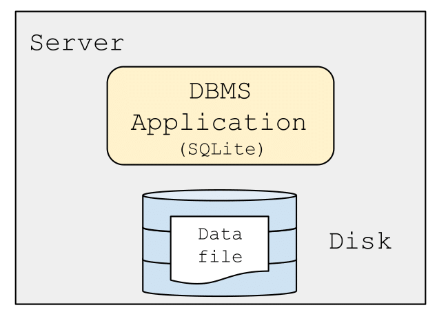
A “single-tier” architecture: one server contains both the database (file) and the application
Two-tier architecture
The need to support multiple simultaneous applications led to the emergence of client-server architecture. In this setup, there is a single database server (typically on a powerful server or cloud service) that is accessed by multiple applications. Each application (referred to as a client) connects to the database using an application programming interface like JDBC or ODBC. Because the actions of these multiple applications may conflict with one another, transactions are imperative to maintain consistency of the database. This architecture permits a larger number of applications to access the same database, and enables higher transaction throughput (the number of transactions the system is able to serve per unit time). However, there is still just one database server and one application server (per application).
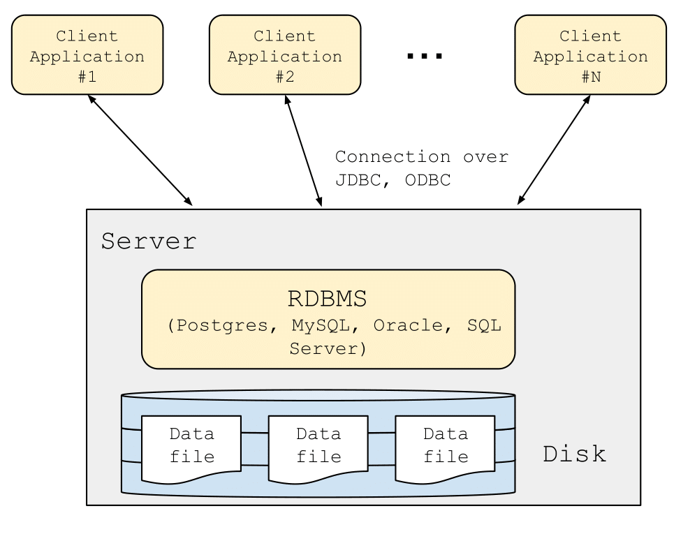 A “two-tier” architecture: the database resides on a single server and multiple client applications connect to it
Three-tier architecture
As one might imagine, one application server is not sufficient to meet the load of modern, global-scale web applications like modern social networks and online stores. In the two-tier architecture the application server is considered the client, so there are maybe 10s of clients connecting to the database. For modern web applications the user’s browser is considered the client, meaning there are 10s to 100s of millions of clients that need to be served. Application servers can be replicated in order to meet this scale. Application servers are relatively easy to replicate because they do not share state (i.e., the only state they need to keep is which clients are connected to them), so it is possible to add 100s or 1000s of new application nodes in order to meet demand. All common state is handled by a database “backend” which communicates with the application servers. This places a high OLTP load on the database, which quickly outstrips the capabilities of a single database server.
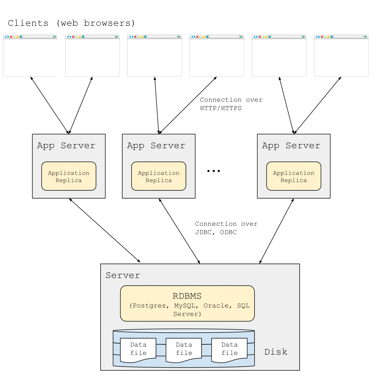 A “three-tier” architecture: database server(s) are distinct from the application frontend servers, which serve user traffic directly. The frontend can be scaled by adding more application servers.
Now we must examine how to scale the database beyond a single server while still providing the consistency required by the OLTP workloads.
Methods for Scaling Databases
Partitioning
The first mechanism we can leverage for scaling a database is partitioning. We have studied partitioning (also called sharding) before when discussing parallel query processing. In order to meet the performance needs of a modern, web-scale application, partitioning becomes extremely useful, as the database can be partitioned into segments of data that are spread out over multiple machines. Performance can increase for two reasons: 1) queries can be executed in parallel on multiple machines if they touch different parts of the database and 2) partitioning the database may allow each partition to fit into memory, which can reduce the disk I/O cost for executing queries. Partitioning can be effective for write-heavy workloads, as query write operations such as inserts and updates, will likely involve writing to just a single machine. However, read-heavy workloads may suffer when queries access data spanning multiple machines (e.g. consider a join on relations partitioned across many machines, requiring costly network transfer), which can decrease performance in comparison to the single database server model.
Replication
Replication is motivated not only by the need to scale the database, but also for the database (and by association the application dependent on accessing the database) to be resilient to failures and extensive down-time where the machine is unresponsive. In all of the 3 architectures studied in Section 2, the database server is a single point of failure, a component that upon failure stops the entire system from functioning. With replication, the data is replicated on multiple machines. This is effective for read-heavy workloads, as queries that read the same data can be executed in parallel on different replicas. However, as the number of replicas increases, writes become increasingly expensive, as queries that update data must now write to each replica of the data to keep them in sync. For each partition, there is a main/primary (formerly called master) copy and duplicates/replicas that are kept in sync.
Partitioning and replication are often used together in real systems to leverage the performance benefits and to make the system more fault-tolerant. As the system scales with more replicas and more partitions, it becomes important to ask questions about how the system will respond when machines begin to fail and the network makes no guarantees about ordering or even the successful delivery of messages.
CAP Theorem
When designing distributed systems, there are three desirable properties that we define here:
-
Consistency: The distributed systems version of consistency is a different concept from the consistency found in ACID. The C in ACID refers to maintaining various integrity constraints of a relational database, such as ensuring that a table’s primary key constraint is satisfied. On the other hand, consistency in the distributed systems context refers to ensuring that two clients making simultaneous requests to the database should get the same view of the data. In other words, even if each client connects to a different replica, the data that they receive should be the same.
-
Availability: For a system to be available, every request must receive a response that is not an error, unless the user input is inherently erroneous.
-
Partition Tolerance: A partition tolerant system must continue to operate despite messages between machines being dropped or delayed by the network, or disconnected from the network altogether.
The CAP theorem (also known as Brewer’s Theorem)3 proves that it is impossible for a distributed system to simultaneously provide more than two of the three (CAP) properties defined above.4 In reality, it is almost impossible to design a system that is completely safe from network failures, and thus most systems must be designed with partition tolerance in mind. The tradeoff then comes between choosing consistency or availability during these periods where the network is partitioned. It is important to note that if there is no network failure, it is possible to provide both consistency and availability.
A system that chooses consistency over availability will return an error or time-out if it cannot ensure that the data view it has access to contains the most recent updates. On the other hand, a system that chooses availability over consistency will always respond with the data view it has access to, even if it is unable to ensure that it contains the most recent updates. In a system that chooses availability over consistency, it is possible that two clients that send a simultaneous read request to different replica machines will receive different values in the event of a network failure that prevents messages between those two replicas. As a concrete example contrasting the two system design choices outlined above, consider a client reading from a replica that cannot access the main copy/replica (due to a network failure). The client will either receive an error (prioritizing consistency) or a stale copy (prioritizing availability).
In fact many such systems provide eventual consistency instead of consistency, in order to trade off availability and consistency. Eventual consistency guarantees that eventually all replicas will become consistent once updates have propagated throughout the system. Eventual consistency allows for better performance, as write operations no longer have to ensure that the update has been successful on all replicas. Instead, the update can be propagated to the rest of the replicas asynchronously. This does lead to a concern about how simultaneous updates at different replicas are resolved, but this is beyond the scope of this class.
So given the difficulty in scaling relational systems, application designers started looking into alternate data models, and that’s where NoSQL comes in.
NoSQL Data Models
NoSQL data stores encompass a number of different data models that differ from the relational model.
Key-Value Stores
The key-value store (KVS) data model is extremely simple and consists only of (key, value) pairs to allow for flexibility. The key is typically a string or integer that uniquely identifies the record and the value can be chosen from a variety of field types. It is typical for a KVS to only allow for byte-array values, which means the application has the responsibility of serializing/deserializing various data types into a byte-array. Due to the flexibility of the KVS data model, a KVS cannot perform operations on the values, and instead provides just two operations: get(key) and put(key, value). Examples of popular key-value stores used in industry include AWS’s DynamoDB, Facebook’s RocksDB, and Memcached.
Wide-Column Stores
Wide-column stores (or extensible record stores) offer a data model compromise between the structured relational model and the complete lack of structure in a key-value store. Wide-column stores store data in tables, rows, and dynamic columns. Unlike a relational database, wide-column stores do not require each row in a table to have the same columns. Another way to reason about wide-column stores is as a 2-dimensional key-value store, where the first key is a row identifier used to find a particular row, and the second key is used to extract the value of a particular column. The data model has two options:
-
key = rowID, value = record
-
key = (rowID, columnID), value = field
The only operations provided are the same as a KVS: get(key) (or get(key, [columns]), which can be thought of as performing a projection on the record) and put(key, value). A couple of the most popular wide-column stores used in industry include Apache Cassandra and Apache HBase (which is based on Google’s BigTable).
Document Stores
In contrast with key-value stores, which are the least-structured NoSQL data model, document stores are among the most structured. The “value” in key-value stores is often a string or byte-array (called unstructured data): this is maximally flexible (you can store anything in a byte array), but often it can be helpful to adopt some convention. This is referred to as semi-structured data. Key-value stores whose values adhere to a semi-structured data format such as JSON, XML or Protocol Buffers are termed document stores; the values are called documents. Relational databases store tuples in tables; document databases store documents in collections.
Document vs Relational Data Models
Recall that the relational data model organizes length-\(n\) tuples into unordered collections called tables, which are described by a set of attributes; each attribute has a name and a datatype. Document data models, on the other hand, can express more complex data structures such as maps/dictionaries, list/arrays and primitive data types, which may be arranged into nested structures. Structured data formats used in document stores include (but are not limited to) Protocol Buffers5, XML6 and JSON.7
One should think of these data formats as just that — formats. They are all ways of serializing the data structures used in applications into a form that can be transmitted over a network and used by client-side code to implement application logic. XML and Java “grew up together” in the early days of the public internet as the dominant data serialization protocol and application programming language, respectively. It was very easy to convert Java objects into XML documents that could be sent over a network and turned back into Java objects on the other side. JSON has grown in popularity along with the JavaScript programming language over the course of the past two decades, and is the predominant data format used by web applications. Protocol Buffers were developed by Google to meet their internal needs for a data serialization format that was smaller and more efficient than XML.
These data formats were originally developed as ways of exchanging data, but are increasingly being used as the data model for document databases. Microsoft’s SQL server supports XML-valued relations; Postgres supports XML and JSON as attribute types; Google’s Dremel supports storing Protobuf; CouchBase, MongoDB, Snowflake and many others support JSON.
JSON Overview
JSON is a text format designed for human-readable and machine-readable interchange of semi-structured data. Originally developed to support exchange of data between a web server and Javascript running in a client’s browser, it is now used as a native representation within many NoSQL databases. Due to its widespread adoption, we will focus on JSON in this class. JSON supports the following types:
-
Object: collection of key-value pairs. Keys must be strings. Values can be any JSON type (i.e., atomic, object, or array). Objects should not contain duplicate keys. Objects are denoted using “{“ and “}” in a JSON document.
-
Array: an ordered list of values. Values can be any JSON type (i.e. atomic, object, or array). Arrays are denoted using “[” and “]” in a JSON document.
-
Atomic: one of a number (a 64-bit float), string, boolean or
null.
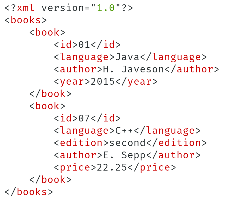 A JSON and XML representation of the same object
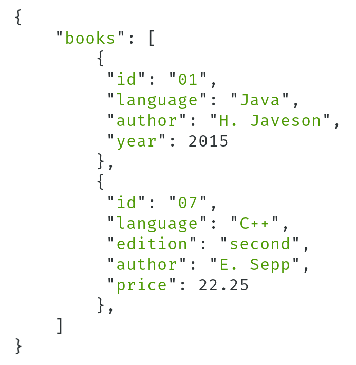
A JSON document consists of one of the above types, which may in turn include nested components. For example, the JSON document in the previous figure consists of an object with a single key ("books"); the value associated with this key is an array of objects. A JSON document can be interpreted as a tree, as in the next figure; this is due to the nested structure of JSON documents.
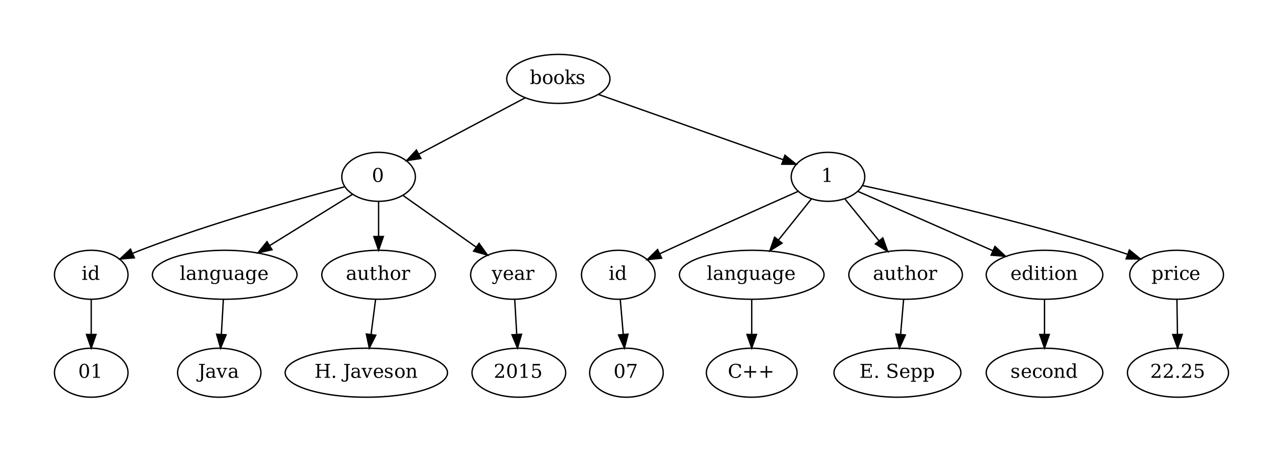 The JSON document in the figure represented as a tree
Another important characteristic of JSON is that it is self-describing — that is, the schema elements are part of the data itself. This allows each document to have its own schema, even within the same document database.
JSON vs Relational
Now we can more directly compare document data model (as typified by JSON) with the relational data model.
-
Flexibility: JSON is a very flexible data model that can easily represent complex structures, including arbitrarily nested data. The relational model is less flexible; it requires keys and joins to represent complex structures.
-
Schema Enforcement: JSON documents are self-describing; each document in a collection can potentially have a unique structure. Under the relational model, the schema for a table is fixed and all tuples in the table must adhere to the pre-defined schema.
-
Representation: JSON is a text-based representation, appropriate for exchange over the web. While it is not necessarily the most efficient representation, it can be easily parsed and manipulated by many different applications and programming languages. In contrast, relational data uses a binary representation which is specialized for a particular database system implementation. It is designed for efficient storage and retrieval from disk — not for sharing information. For instance, MySQL and Postgres each have their own binary data format that are mutually incompatible.
Note that there are intermediate representations such as TSON (typed-JSON) and BSON (binary-JSON) which can enforce schema restrictions or have binary representations that are more efficient than standard JSON; we omit them for this discussion.
As always, there are tradeoffs to be made. We review two of them here.
First, relational databases trade flexibility for simplifying application code. Relational databases are sometimes described as “enforcing schema on write”, and document databases are sometimes described as “enforcing schema on read”. Applications querying a relational database will know exactly the structure and data types of the rows that are returned; this can be determined through examining the schemas of the tables being queried. However, applications querying a document database will need to inspect the schema of each document in a collection, which pushes complexity into the application logic. We will investigate this in more detail in Section 5.4 below.
Second, the document model is more suitable for data which is primarily accessed by a primary key (like an email or user ID). For these kinds of lookups, the document model exhibits better locality; all the data related to the key of interest can be returned in a single query. This is typically more efficient for a document database than for a relational database: information could be stored in multiple tables and require several joins in order to retrieve the same information.
Converting Between JSON and Relational
Some relational databases such as Postgres and SQLite permit the storage and querying of JSON in a relational context; a table attribute can have a type of JSON and elements of the JSON document can be retrieved or queried through the use of special operators and functions. It is also possible to transform JSON documents into a form that can be represented in the relational model, and vice versa.
Transforming Relational to JSON: A single table with a set of attributes can be represented in JSON as an object whose key is the name of the table and whose value is an array of objects. Each object in the array corresponds to a row in the table: the object has the table attributes as keys, and the tuple elements as values. A table with foreign keys into another table (a one-to-many relationship) can be represented in JSON as a nested structure for which the linked rows in the second table are embedded or “inlined” into the objects representing the row of the first table.
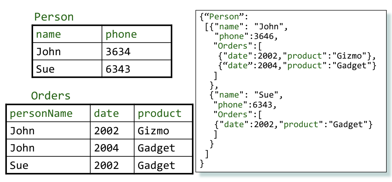 A JSON representation of relational tables
Many-to-many relationships in a relational schema are harder to represent without introducing duplicate data. Consider a set of three relations, one of which has foreign keys into two other primary-keyed tables (this is the relationship table). There are three options for representing this setup using JSON. The first option is to represent each relation as a flat JSON array (where each element is an object representing a row); this has no redundant data, but relies on the application to join the tables to get related data. The second and third options key off of the one of the primary-keyed tables and inlines the contents of the relationship table and the last table within each object. In either of these cases, the elements of the last table will be duplicated for each linked element of the first table. This redundancy means that the application does not need to perform any joins to get the full record (because it is all stored in the same document), but also means that updates to the document store will need to handle updating all duplicated rows.
Transforming JSON to Relational: Representing semi-structured data as a relation can be tricky because of the potential variation in structure of the documents at hand. Consider the document in the figure. This suggests a relational table person(name, phone, address, email), but there are several issues. First, one of the objects in our JSON document has two phone numbers; the schema would need to factor phone numbers out into another table, or suffer the inclusion of duplicate data. Second, one of the objects has an email but another does not. The relational schema can represent the absence of an email with a NULL value in the table, but what if future documents contain additional attributes? The schema of the table would need to be changed, which is a potentially expensive manual process. Lastly, the address fields of the two objects have different structures: one contains a simple string and the other contains a nested object. There is no obvious “best” way to represent these two structures in a relational database.
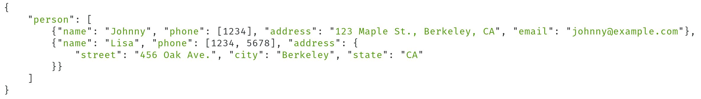 A JSON document which is difficult to translate to a relational table
Querying Semi-Structured Data
Semi-structured data models have their own set of query languages, distinct from SQL. These query languages must handle the variety of structures found in semi-structured data: repeated attributes, different types for the same attributes, nested and heterogeneous collections, and so on. We studied one such language in class (the MongoDB query language), and provide a brief summary here. See class lecture slides or the manual8 for more details.
Retrieval queries: A retrieval query in MongoDB generally matches the following form:
db.collection.find(<predicate>, optional <projection>)
It returns any documents in collection that match <predicate> while keeping the fields as specified in <projection>. Both <predicate> and <projection> are expressed as documents! For example, a query to find all documents with category food could be expressed as find({category:"food"}) and one to find all the documents with a quantity \(\geq 50\) could be expressed as find({qty:{$$gte:50}}). Just like $$gte, there are other keywords such as $$elemMatch and $$or that can be used to express even more complex queries.
The output of a retrieval query can be further customized by limiting the number of returned results or ordering them in a certain way (just like SQL). Here is an example of a query that limits the number of returned documents and then sorts the results by quantity.
db.collection.find({category:"food"}).limit(10).sort({qty:1})
Other queries: MongoDB’s query language also supports more complicated query pipelines (called aggregation pipelines) as well as updates and deletions. These follow the same document-based syntax and offer a lot of flexibility.
Problems
-
Are the following workloads better characterized as Online Transaction Processing (OLTP) or Online Analytical Processing (OLAP)?
-
Placing orders and buying items in an online marketplace
-
Analyzing trends in purchasing habits in an online marketplace
-
-
Earlier in this class, we learned about the Two Phase Commit protocol. In relation to the CAP theorem, which of the CAP properties (consistency, availability, partition tolerance) does 2PC choose, and which does it give up?
-
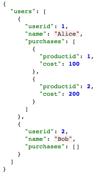
Suppose we would like to translate the following data from the relational model to JSON in migrating to a NoSQL database like MongoDB. Given that we want to be able to list all purchases a user made without performing any joins or aggregations, what will the resulting JSON document look like?
Users
userid username 1 “alice” 2 “bob” Purchases
userid productid cost 1 1 100 1 2 200
Solutions
-
-
OLTP: OLTP workloads involve high numbers of transactions executed by many different users. Queries in these workloads involve simple lookups more often than complex joins. In this case, when a user buys an item, the site might perform actions like looking up the item and updating its quantity, recording a new purchase, etc.
-
OLAP: OLAP workloads involve read-only queries and typically include lots of joins and aggregations. Often, workloads executed for analysis and decision making are OLAP workloads.
-
-
2PC chooses consistency and partition tolerance, and gives up on availability. By enforcing that a distributed transaction either commits or aborts on all nodes involved, it guarantees that these nodes will provide consistent views of the data. However, we cannot provide all three of the CAP properties, and we give up on availability. For example, consider what happens to participants who voted yes if the coordinator crashes - they will be stuck in a state of limbo, waiting to learn about the status of the transaction and holding their locks under strict 2PL. If other transactions try to access the data these locks are held on, they will end up on a wait queue; hence, this data is unavailable.
- To avoid performing joins when finding all purchases for a user, we can inline Purchases within Users, storing a list of purchases for each user.
-
and also old, as we will see. ↩
-
Seymour Cray famously asked “"If you were plowing a field, which would you rather use? Two strong oxen or 1024 chickens?” ↩
-
The CAP theorem was first presented as a conjecture by Eric Brewer in 1998 and later formally proved by Seth Gilbert and Nancy Lynch in 2002. ↩
-
For a concise, illustrated proof of the CAP theorem written by a former TA, refer to https://mwhittaker.github.io/blog/an_illustrated_proof_of_the_cap_theorem/ ↩
-
Also called “protobuf”: https://developers.google.com/protocol-buffers ↩
-
Extensible Markup Language: https://www.w3.org/XML/ ↩
-
JavaScript Object Notation: https://www.json.org ↩