Introduction
In previous modules, we learned how to parallelize relational database systems which is useful for optimizing data processing but only works well up to a certain number of machines. Difficulties and headaches come when we start thinking about scaling the relational model on databases split across hundreds or thousands of machines. This became a problem when more and more people, especially every day consumers, started to interact with databases when the Internet exploded around the turn of the 21st century. Database thinking, models, and technologies needed to catch up to meet the demand. This note will focus on two recent advances in parallel database technologies - MapReduce and Spark - that have enabled the massive scalability of modern data processing.
MapReduce
DFS and High-Level Introduction
Engineers at Google in the early 2000s needed a way to efficiently manage and process the large amounts of data (at petabyte scale and beyond) that was being generated, stored, and indexed by the company. First off, they needed a way to store files across hundreds and eventually thousands of machines since only a few would definitely not be enough. To do this, they designed a file system in which large files (TBs, PBs) are partitioned into smaller files called chunks (usually 64MB) and then distributed and replicated several times on different nodes for fault tolerance. This is called a distributed file system (DFS) which has had countless implementations since then from Google’s proprietary GFS to Hadoop’s open source HDFS.
Next, they needed a way to efficiently process the large amount of data stored on a DFS. To do this, they built MapReduce which is a high-level programming model and implementation for large-scale parallel data processing. Its name is derived from the two main and separate phases of the process: Map and Reduce. From a high level, we can describe the Map phase as applying a function in parallel to every element of a set of data and the Reduce phase as combining the results of the Map phase into the desired data output. The magic of this paradigm in processing data at scale is it automatically handles the details of issuing and managing tasks in parallel across multiple machines. A user only has to define the Map and Reduce tasks and MapReduce takes care of the rest, similar to how SQL creates an execution plan from a query.
Data Model and Programming
The data model in MapReduce works on files called bags, which contain pairs. A MapReduce program takes in an input of a bag of pairs and outputs a bag of pairs ( is optional). The user must provide two stateless functions – and – to define how the input pairs will be transformed into the output pair domain.
The first part of MapReduce – the Map phase – applies a user-provided Map function in parallel to an input of pairs and outputs a bag of pairs. The types and values of , , , and are independent of each other. The pairs serve as intermediate tuples in the MapReduce process.
func map(key1, value1) -> bag((key2, value2))
The second part of MapReduce – the Reduce phase – groups all intermediate pairs outputted by the Map phase with the same and processes each group into a single bag of output values defined by a user-provided Reduce function. This function is also run in parallel with a machine or worker thread processing a single group of pairs with the same . The pairs in this function serve as the output tuples in the MapReduce process.
func reduce(key2, bag(value2)) -> bag((key3, value3))
Word Count Example
Let’s start with an example of counting the number of occurrences of each word in a large collection of documents. Each document is a bag of key-value pairs with key being the document and value being the entire set of words in that document.
We define the following map function to emit an intermediate pair for every word that appears in a document. Note that this function is stateless so we can run it in parallel.
map(String key, String value):
    // key: document name
    // value: document contents
    for each word w in value:
        emitIntermediate(w, 1)
After applying this map function to all documents, we essentially have a collection of all individual words that appear in all documents with a 1 assigned to each to represent the number of appearances. For example:
(apple, 1)
(banana, 1)
(banana, 1)
(book, 1)
…
(shoe, 1)
MapReduce then groups intermediate pairs with the same word key and for each group, combines their values (in this case all 1s) into an iterator. The following reduce function takes the iterator for each word key and returns the sum over the 1s in the values, resulting in the count of each word across all documents.
reduce(String key, Iterator values):
    // key: a word
    // values: a list of counts
    int sum = 0;
    for each v in values:
        sum += v;
    emit(key, sum);
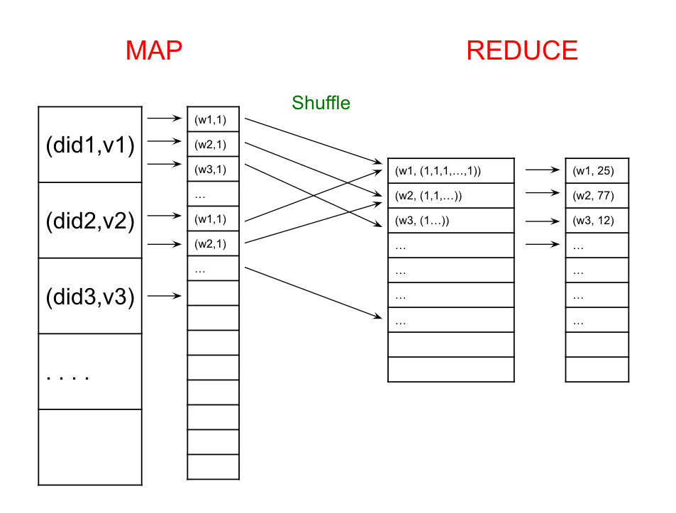
Here is a visual diagram of what happens at a high level in MapReduce. First, we map each document to a list of (word, 1) pairs. Then, we shuffle (or group) these intermediate pairs based on the word and create a list of 1s for each group. Final, the reduce function sums over this list to generate the word count for each word.
Workers
MapReduce processes are split up and run by workers which are processes that execute one task at a time. With 1 worker per core, we can have multiple workers per node in our system.
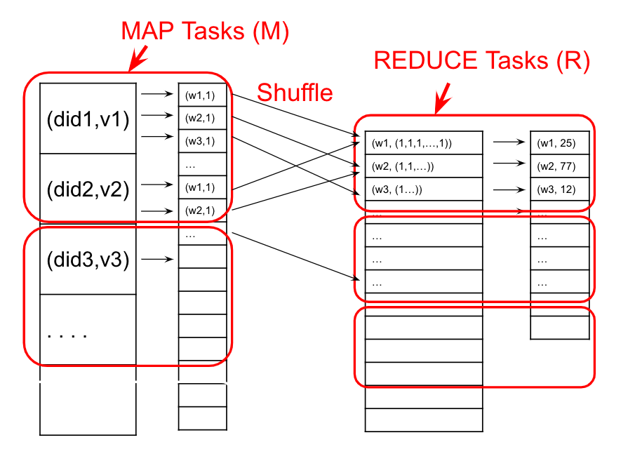
Here is the same Word Count example but with worker tasks denoted by what part of the MapReduce process they handle. Both the Map and Reduce phases can be split among different workers on different machines, with workers performing independent tasks in parallel. Also, the shuffling process here is automatically handled by the system.
Implementation
Like 2PC, MapReduce designates one machine as the leader node. Its role is to accept new MapReduce tasks and assign them to workers later on. The leader begins by partitioning the input file into \(M\) splits by key and assigning workers to \(M\) map tasks, keeping track of progress as workers perform their tasks. Workers write their output to the local disk and partition their output into \(R\) regions. The leader then assigns workers to the \(R\) reduce tasks which then write the final output to disk once complete.
Fault Tolerance
Now, we can start thinking of possibilities of failure in this implementation. One of the most common faults is the failure of a worker performing a map task. One way to solve this is to just restart a new mapper task and read the data it is supposed to process from the disk again. However, since the Reduce phase must wait until the entire Map phase completes, does this mean if one map task fails then we must restart the entire Map phase again?
No. If we write the intermediate result of the Map phase to disk, then we can avoid this. This means that the Reduce phase workers will have to read files from disk as its input and exactly like the Map phase workers - if one crashes during execution, it just gets restarted.
Another interesting detail about the MapReduce implementation is how it handles machines that take an unusually long time to complete one of its tasks, also known as a straggler. These stragglers could be the result of faulty hardware, too many tasks assigned to one machine, or any number of other reasons. To avoid this, MapReduce preemptively starts new executions of the last few remaining in-progress tasks, with the hope that all the necessary tasks are completed.
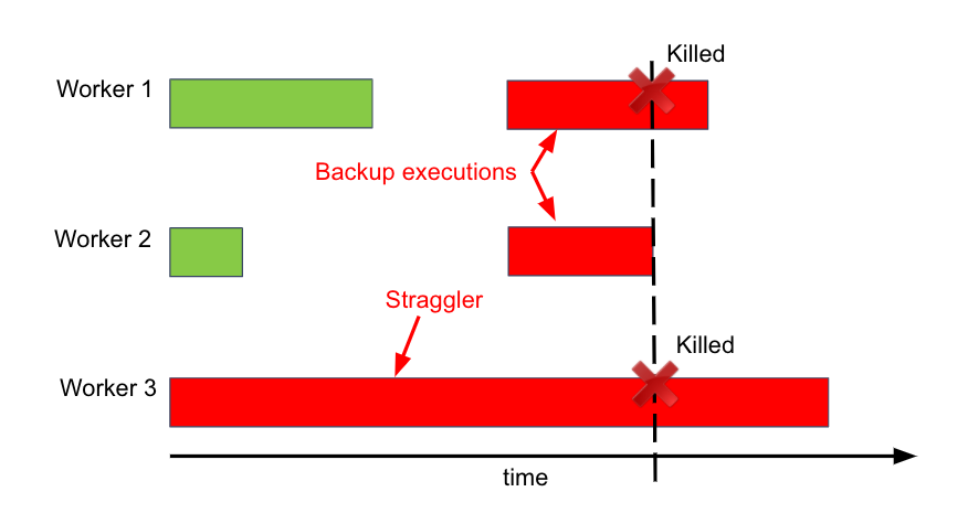
For example, in this case of 3 workers, worker 1 and 2 complete their tasks first while worker 3 straggles. MapReduce then decides to utilize worker 1 and 2, which are now idle, to start the same task as worker 3 as backup. Once worker 2 finishes this task, the remaining tasks on worker 1 and 3 are killed and the MapReduce process can proceed.
Selection, Group By, Join
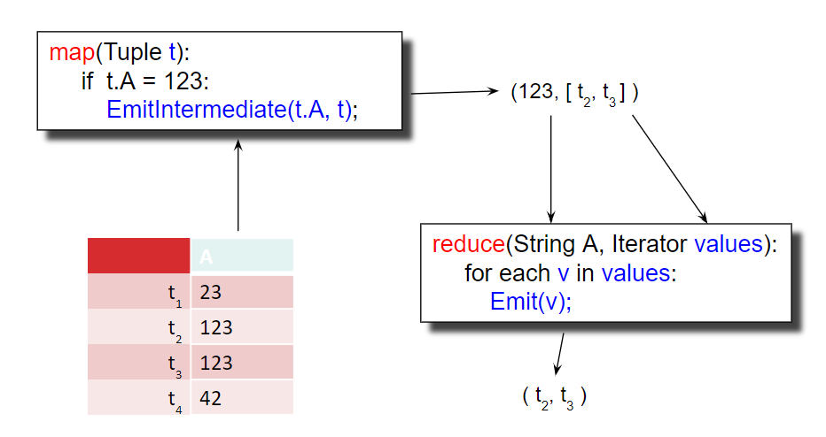
Let’s look at how to implement a selection (from relational algebra) using MapReduce. If we want to perform a query like \(\sigma_{A=123}{(R)}\), our map and reduce functions are:
map(Tuple t):
    if t.A = 123:
        EmitIntermediate(t.A, t);

reduce(String A, Iterator values):
    for each v in values:
        Emit(v);
The map function is applied over all the data and only outputs tuples if their A field = 123. The reduce function just serves to output the tuples in the end. While the reduce function is arguably unnecessary in this case, we must always supply both the map and reduce functions to MapReduce.\
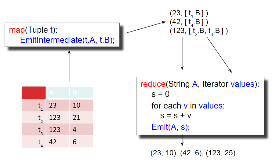
Moving on, to implement a group by operator such as \(\gamma_{A, sum(B)}{(R)}\), our map and reduce functions are:
map(Tuple t):
    EmitIntermediate(t.A, t.B);

reduce(String A, Iterator values):
    s = 0;
    for each v in values:
        s = s + v;
    Emit(A, s);
In the map function, we assign the key of the intermediate pairs as since we are grouping by A and assign the value as since we want to sum over the B values. In the reduce function, we do just that as we iterate over the B values of each of the group.\
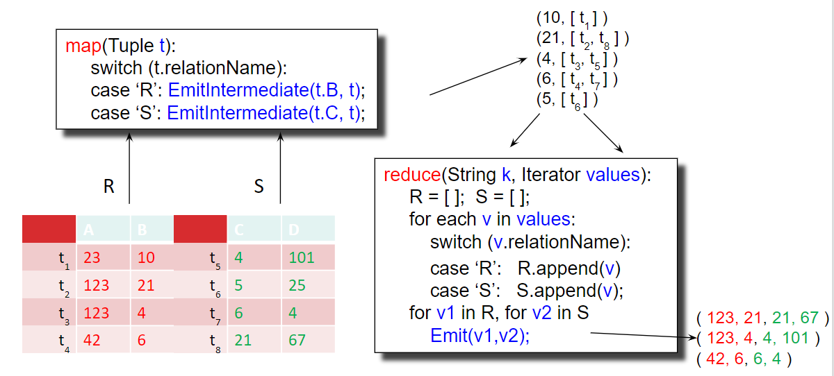
Finally, let’s tackle the more challenging yet still practical implementation of a inner join using MapReduce. If we have relations \(R(A, B)\) and \(S(C, D)\) and want to perform the inner join \(R \bowtie_{B=C} S\), we need to be a bit more clever in how we structure our map and reduce functions. For our map function, we need to output intermediate pairs such that tuples from R will be matched with tuples from S on R.B = S.C and whose source table is stored. These pairs will be grouped by the matching R.B = S.C values and will then need to be processed by a reduce function which can separate tuples by their source tables, create two separate lists, and output each pair from the two lists. These map and reduce functions do just that:
map(Tuple t):
    switch (t.relationName):
    case 'R': EmitIntermediate(t.B, t);
    case 'S': EmitIntermediate(t.C, t);

reduce(String k, Iterator values):
    R = []; S = [];
    for each v in values:
        switch (v.relationName):
        case 'R': R.append(v)
        case 'S': S.append(v);
    for v1 in R, v2 in S:
        Emit(v1, v2);
Spark
History and Motivation
We’ve seen how MapReduce provides a high-level programming paradigm to handling scalable, distributed, fault-tolerant data processes across many machines. However, it comes with several drawbacks and limitations:
-
As mentioned previously, users must always provide both the map and the reduce functions. With such a strict format, it can be difficult to write more complex queries.
-
Writing intermediate results to disk is necessary for fault tolerance, but can be very slow.
-
Running multiple MapReduce jobs can take a long time due to waiting for writes to finish.
Spark was developed right here in Berkeley to address these issues. It is an open source system that handles distributed processing over HDFS like MapReduce. But unlike MapReduce, Spark:
-
Consists of multiple steps instead of 1 mapper + 1 reducer.
-
Stores intermediate results in main memory.
-
Resembles relational algebra more closely.
Resilient Distributed Datasets
Spark’s data model consists of semi-structured data objects called Resilient Distributed Datasets (RDDs). These objects, which can be anything from key value pairs to objects of a certain type, are immutable datasets that can be distributed across multiple machines. For faster execution, RDDs are not written to disk in intermediate steps but are rather stored in main memory. Since this will lead to intermediate results being lost if a node crashes, each RDD’s lineage is tracked which can help recompute RDDs. This means that we must store the lineage in persistent storage, like writing to disk before executing the program, to generate the output RDD. In practice, this can be done by writing to a log and flushing it to the disk, just like what we learned earlier in the Recovery module.
Programming
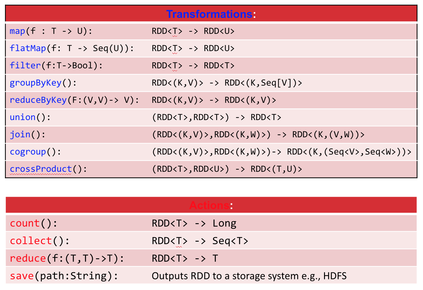
Spark programs consist of two types of operators: transformations and actions. Actions are eager operators which means they are executed immediately when called. These include operators such as count, reduce, and save. Transformations, on the other hand, are evaluated lazily, meaning they are not executed immediately but are rather recorded in the lineage log. An operator tree, similar to a relational algebra tree, is constructed in memory. Transformations were designed this way to optimize operator execution, similar to how SQL optimizes over a set of query plans. For example, if we have two consecutive selections, we can combine them to a single selection to save 1 entire pass over the RDD which saves I/Os. Other transformations include map, reduceByKey, join, and filter.
Now let’s see how Spark is actually programmed. In this example, we are reading a large log as a textfile and want to output all lines that start “NullPointerException" and contain “SQLite":
s = SparkSession.builder()...getOrCreate();
lines = s.read().textFile("hdfs://logfile.log");
nullErrors = lines.filter(l -> l.startsWith("NullPointerException"));
sqlLiteErrors = nullErrors.filter(l -> l.contains("SQLite"));
sqlLiteErrors.collect();
Here, the first line creates a context object that can be used to create RDDs. The second line then reads the log. Filtering on the two conditions is performed by the third and fourth line, but remember this is a transformation so they are not evaluated until we call on the last line which is an action and thus, triggers the computation.
A more concise and arguably cleaner version of this Spark code which better illustrates data flow can be written like this (“call chaining" style):
s = SparkSession.builder()...getOrCreate();
errors = s.read().textFile("hdfs://logfile.log")
    .filter(l -> l.startsWith("NullPointerException"))
    .filter(l -> l.contains("SQLite"))
    .collect();
Persistence
Since Spark does not write intermediate results to disk, if a server fails before a program finishes, the entire execution of that program must restart. However, Spark does allow options to avoid that. If we want to persist, or materialize, our intermediate results, we can call at points in our code like this:
s = SparkSession.builder()...getOrCreate();
lines = s.read().textFile("hdfs://logfile.log");
nullErrors = lines.filter(l -> l.startsWith("NullPointerException"));
nullErrors.persist(); \\ <-- MATERIALIZATION
sqlLiteErrors = nullErrors.filter(l -> l.contains("SQLite"));
sqlLiteErrors.collect();
This will fully compute as an RDD and store the results to disk, essentially creating a checkpoint at which we can restart if the server fails.
Join Example
Let’s convert the following SQL query into Spark code:
SELECT COUNT(*) FROM R, S
WHERE R.B > 200 AND S.C < 100 AND R.A = S.A
We can read in R and S and parse each line into an object, persisting on disk this intermediate result like this:
R = s.read().textFile("R.csv").map(parseRecord).persist();
S = s.read().textFile("S.csv").map(parseRecord).persist();
Then we create our transformations to apply the two single relation conditions in the where clause:
RB = R.filter(t -> t.b > 200).persist();
SC = S.filter(t -> t.c < 100).persist();
To join the two filtered relations, we can simply use Spark’s function:
J = RB.join(SC).persist();
Finally, we apply the like so:
J.count();
A Partial List of Spark Transformations and Actions
Spark 2.0 – DataFrames and Datasets
Spark 2.0 introduced two new forms of data collections: DataFrames and Datasets.
DataFrames are very similar to relations in that each object in a DataFrame is called a Row and have attributes called Columns. They also have more SQL-like API functions such as and . Let’s look at converting the following SQL query to Spark using Datasets (source):
SELECT AVG(p.salary), MAX(p.age)
FROM people p, department d
WHERE p.age > 30 AND p.deptId = d.id
GROUP BY d.name, gender
We can read in the and relations and then chain transformations and actions like so:
Dataset<Row> people = s.read().textFile("R.csv");
Dataset<Row> department = s.read().textFile("S.csv");

people.filter("age".gt(30))
    .join(department, people.col("deptId").equalTo(department("id")))
    .groupBy(department.col("name"), "gender")
    .agg(avg(people.col("salary")), max(people.col("age")));
Datasets are a more general type of DataFrames in which its elements must be typed objects ( rather than ). In fact, DataFrames are just Datasets with object type . Here is a sample of the Datasets API:
agg(Column expr, Column... exprs)
Aggregates on the entire Dataset without groups.

groupBy(String col1, String... cols)
Groups the Dataset using the specified columns, so that we can run aggregation on them.

join(Dataset<?> right)
Join with another DataFrame.

orderBy(Column... sortExprs)
Returns a new Dataset sorted by the given expressions.

select(Column... cols)
Selects a set of column based expressions.
Conclusion
In this note, we looked at two technologies that have been design to perform parallel data processing on the terabyte scale and beyond: MapReduce and Spark. MapReduce came first and utilized user-defined map and reduce functions (hence its name). It writes intermediate results to disk which is great for fault tolerance but bad for I/O cost and performance. It also pioneered the model of automatically assigning, tracking, and managing tasks among workers across many machines and is equipped to handle failures and stragglers.
Spark came along to address some of the issues of MapReduce which include its strict structure, difficulty in writing complex queries, and slow performance due to intermediate writes. Spark uses the object-based Resilient Distributed Dataset (RDD) and is operated by transformations, which are evaluated lazily, and actions, which are evaluated eagerly. Spark more closely resembles relational algebra, has features that allow for persistence, and recently introduced new data models (DataFrames, Datasets) which better resembles the relational data model.
Practice Questions
1. MapReduce is run over 5 worker nodes: M1, M2, M3, M4, and M5. Each machine is given an equal amount of work. All the machines except M5 are given a 10 seconds to finish their task. However, M5 takes 50 seconds because it has fewer hardware resources. How long will this MapReduce job take to finish? Give a best-case and worst-case scenario.
Solutions
1. In the best case, the job will take 20 seconds. Machines M1 through M4 will finish in 10 seconds in parallel. Then, if MapReduce immediately pre-emptively schedules M5’s job on one of M1 through M4, that job will also take another 10 seconds. 10 + 10 = 20 seconds. However, if MapReduce doesn’t immediately pre-emptively reschedule M5’s job, then M5 will certainly finish the job in 50 seconds in parallel with the other machines. Therefore, in the worst case, the job will take 50 seconds.
Past Exam Problems
-
Sp21 Final Q8 pg 34-36
-
Fa20 Final Q1 pg 3