Introduction

In the previous notes, we went over different file and record representations for data storage. This week, we will introduce index which is a data structure that operates on top of the data files and helps speed up reads on a specific key. You can think of data files as the actual content of a book and a index as the table of content for fast lookup. We use indexes to make queries run faster, especially those that are run frequently. Consider a web application that looks up the record for a user in a Users table based on the username during the login process. An index on the username column will make login faster by quickly finding the row of the user trying to log in. In this course note, we will learn about B+ trees, which is a specific type of index. Here is an example of what a B+ tree looks like:

Properties

• The number d is the order of a B+ tree. Each node (with the exception of the root node) must have d ≤ x ≤ 2d entries assuming no deletes happen (it’s possible for leaf nodes to end up with < d entries if you delete data). The entries within each node must be sorted.

• In between each entry of an inner node, there is a pointer to a child node. Since there are at most 2d entries in a node, inner nodes may have at most 2d+1 child pointers. This is also called the tree’s fanout.

• The keys in the children to the left of an entry must be less than the entry while the keys in the children to the right must be greater than or equal to the entry.

• All leaves are at the same depth and have between d and 2d entries (i.e., at least half full)

For example, here is a node of an order d=2 tree:

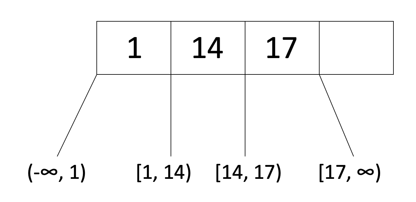
Note that the node satisfies the order requirement, also known as the occupancy invariant (d ≤ x ≤ 2d) because d=2 and this node has 3 entries which satisfies 2 ≤ x ≤ 4.

• Because of the sorted and children property, we can traverse the tree down to the leaf to find our desired record. This is similar to BSTs (Binary Search Trees).

• Every root to leaf path has the same number of edges - this is the height of the tree. In this sense, B+ trees are always balanced. In other words, a B+ tree with just the root node has height 0.

• Only the leaf nodes contain records (or pointers to records - this will be explained later). The inner nodes (which are the non-leaf nodes) do not contain the actual records.

For example, here is an order d=1 tree:

Insertion

To insert an entry into the B+ tree, follow this procedure:

1. Find the leaf node L in which you will insert your value. You can do this by traversing down the tree. Add the key and the record to the leaf node in order.

2. If L overflows (L has more than 2d entries)

   1. Split into L_1 and L_2. Keep d entries in L_1 (this means d+1 entries will go in L_2).

   2. If $L$ was a leaf node, COPY $L_2$’s first entry into the parent. If $L$ was not a leaf node, MOVE $L_2$’s first entry into the parent.

   3. Adjust pointers.

3. If the parent overflows, then recurse on it by doing step 2 on the parent. (This is the only case that increases the tree height)

Note: we want to COPY leaf node data into the parent so that we don’t lose the data in the leaf node. Remember that every key that is in the table that the index is built on must be in the leaf nodes! Being in a inner node does not mean that key is actually still in the table. On the other hand, we can MOVE inner node data into parent nodes because the inner node does not contain the actual data, they are just a reference of which way to search when traversing the tree.

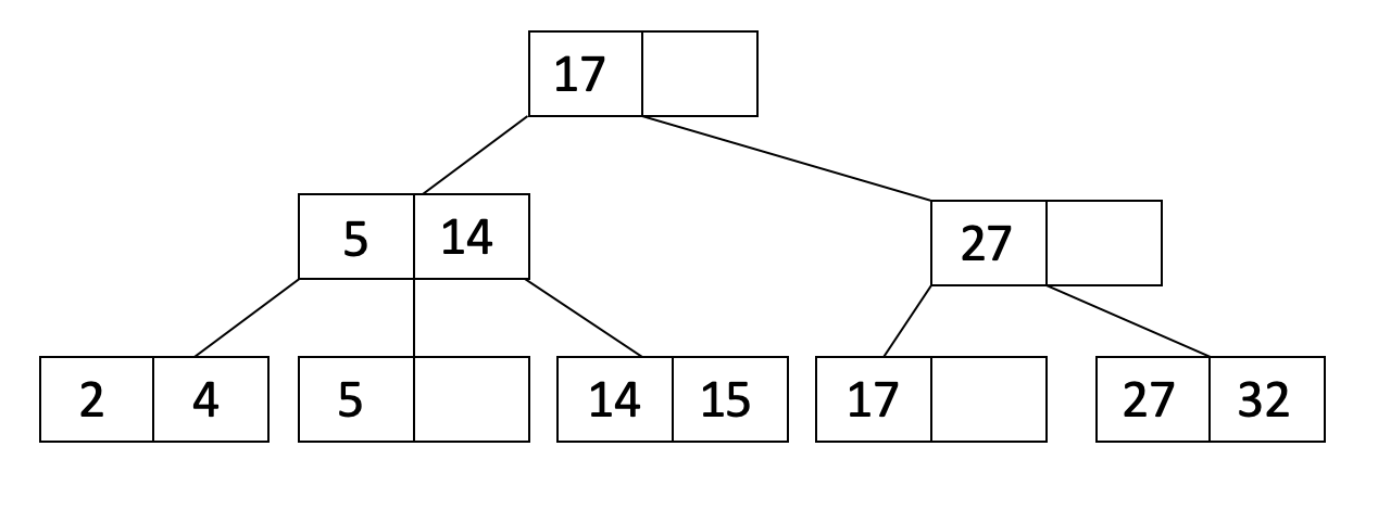
Let’s take a look at an example to better understand this procedure! We start with the following order d=1 tree:

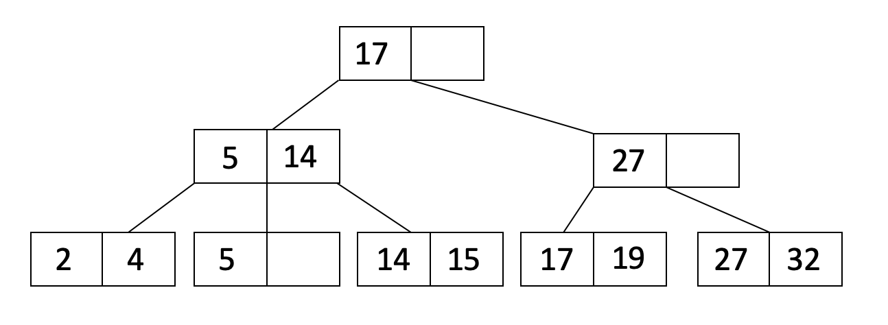
Let’s insert 19 into our tree. When we insert 19, we see that there is space in the leaf node with 17:

Now let’s insert 21 into our tree. When we insert 21, it causes one of the leaf nodes to overflow. Therefore, we split this leaf node into two leaf nodes as shown below:

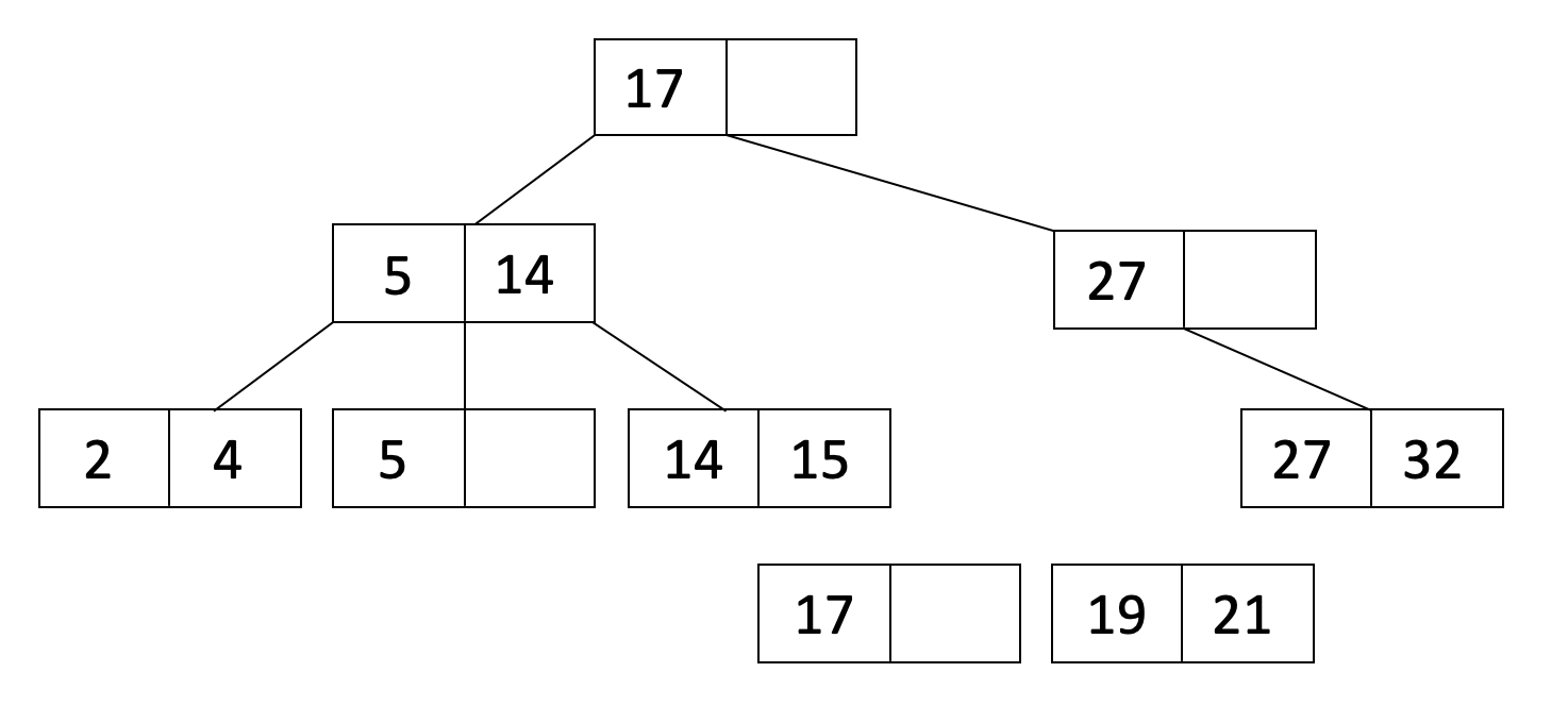
L_1 is the leaf node with 17, and L_2 is the leaf node with 19 and 21.

Since we split a leaf node, we will COPY L_2’s first entry up to the parent and adjust pointers. We also sort the entries of the parent to get:

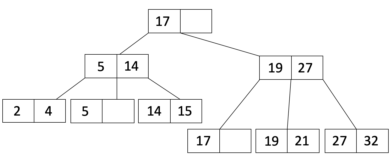
Let’s do one more insertion. This time we will insert 36. When we insert 36, the leaf overflows so we will do the same procedure as when we inserted 21 to get:

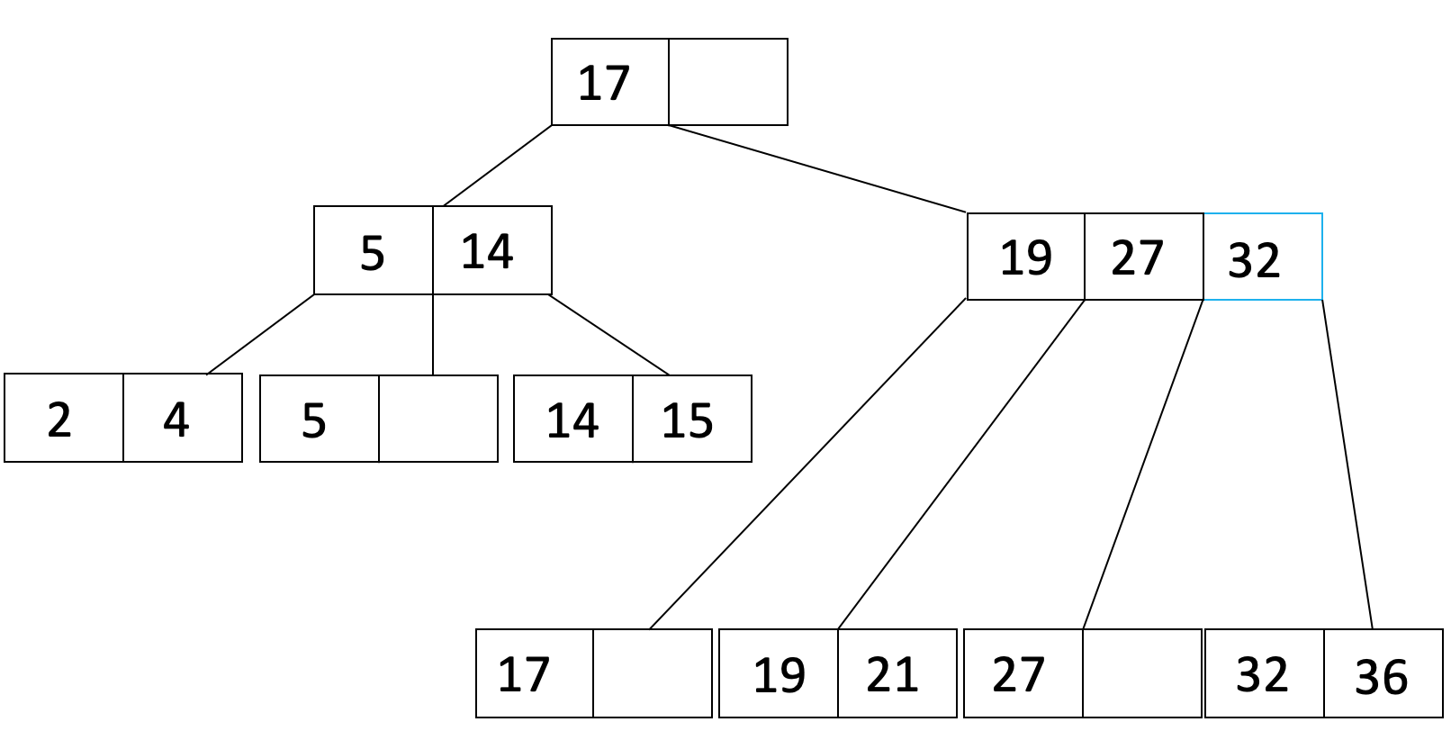
Notice that now the parent node overflowed, so now we must recurse. We will split the parent node to get:

L_1 is the inner node with 19, and L_2 is inner the node with 27 and 32.*

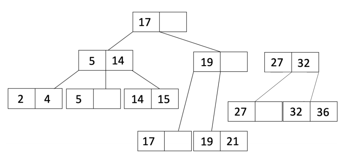
Since it was an inner node that overflowed, we will MOVE L_2’s first entry up to the parent and adjust pointers to get:

Lastly, here are a couple clarifying notes about insertion into B+ Trees:

• Generally, B+ tree nodes have a minimum of d entries and a maximum of 2d entries. In other words, if the nodes in the tree satisfy this invariant before insertion (which they generally will), then after insertion, they will continue to satisfy it.

• Insertion overflow of the node occurs when it contains more than 2d entries.

Deletion

To delete a value, just find the appropriate leaf and delete the unwanted value from that leaf. That’s all there is to it. (Yes, technically we could end up violating some of the invariants of a B+ tree. That’s okay because in practice we get way more insertions than deletions so something will quickly replace whatever we delete.)

Reminder: We never delete inner node keys because they are only there for search and not to hold data.

Storing Records

Up until now, we have not discussed how the records are actually stored in the leaves. Let’s take a look at that now. There are three ways of storing records in leaves:

• Alternative 1: By Value

  In the Alternative 1 scheme, the leaf pages are the data pages. Rather than containing pointers to records, the leaf pages contain the records themselves.

  Points	Name
  2	MEM
  3	LAK
  5	BOS
  7	MIL
  20	BKL
  24	GSW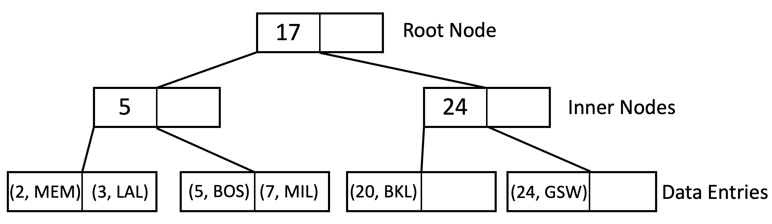

  

  While the Alternative 1 Scheme is perhaps the easiest implementation, it has a significant limitation: if all we have is the Alternative 1 Scheme, we cannot support multiple indexes built on the same file (in the example above we cannot support a secondary index on ‘name’. Instead we would have to duplicate the file and build a new Alternative 1 index on top of that file.

• Alternative 2: By Reference

  In the Alternative 2 scheme, the leaf pages hold pointers to the corresponding records.

  Points	Name
  2	MEM
  3	LAK
  5	BOS
  7	MIL
  20	BKL
  24	GSW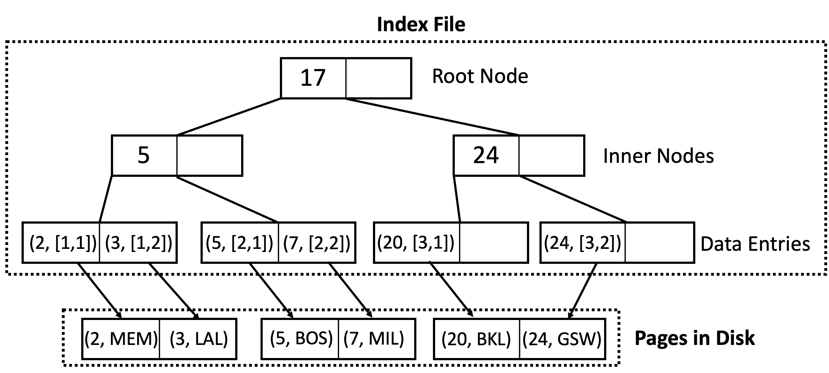

  

  Notation Clarification: In the diagram above, the leafs contain (Key, RecordID) pairs where the RecordID is [PageNum, RecordNum].

  Indexing by reference enables us to have multiple indexes on the same file because the actual data can lie in any order on disk.

• Alternative 3: By List of References

  In the Alternative 3 scheme, the leaf pages hold lists of pointers to the corresponding records. This is more compact than Alternative 2 when there are multiple records with the same leaf node entry. Each leaf now contains (Key, List of RecordID) pairs.

  Points	Name
  2	MEM
  2	LAK
  2	BOS
  7	MIL
  7	BKL
  50	GSW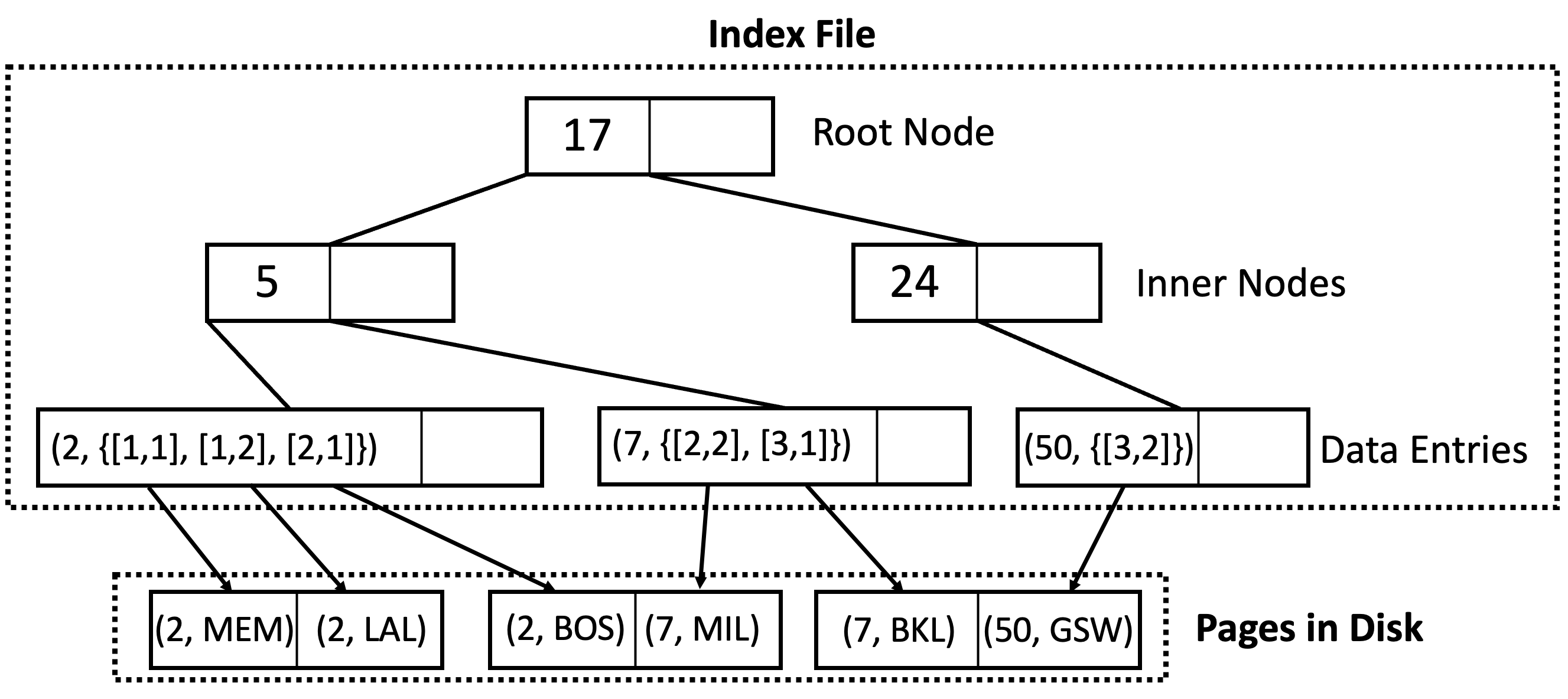

  

Clustering

Now that we’ve discussed how records are stored in the leaf nodes, we will also discuss how data on the data pages are organized. Clustered/unclustered refers to how the data pages are structured. Because the leaf pages are the actual data pages for Alternative 1 and keys are sorted on the index leaf pages, Alternative 1 indices are clustered by default. Therefore, unclustering only applies to Alternative 2 or 3.

• Unclustered

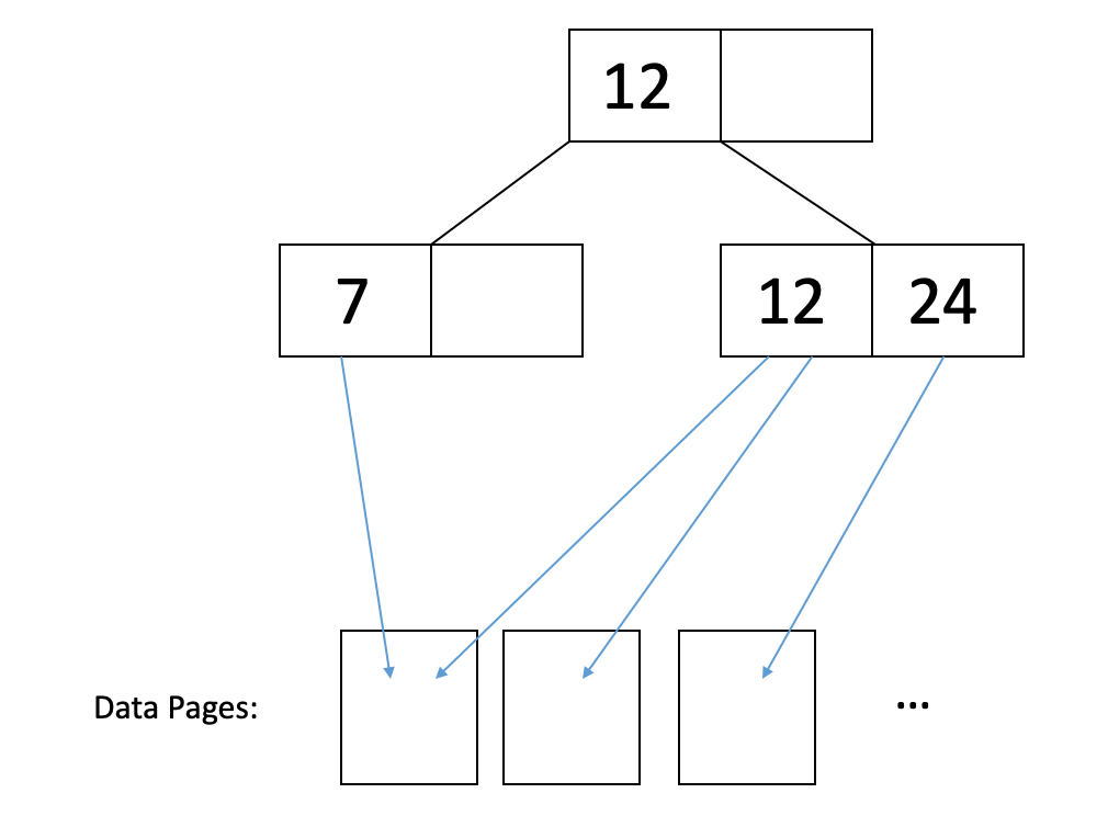
  In an unclustered index, the data pages are complete chaos. Thus, odds are that you’re going to have to read a separate page for each of the records you want. For instance, consider this illustration:

  

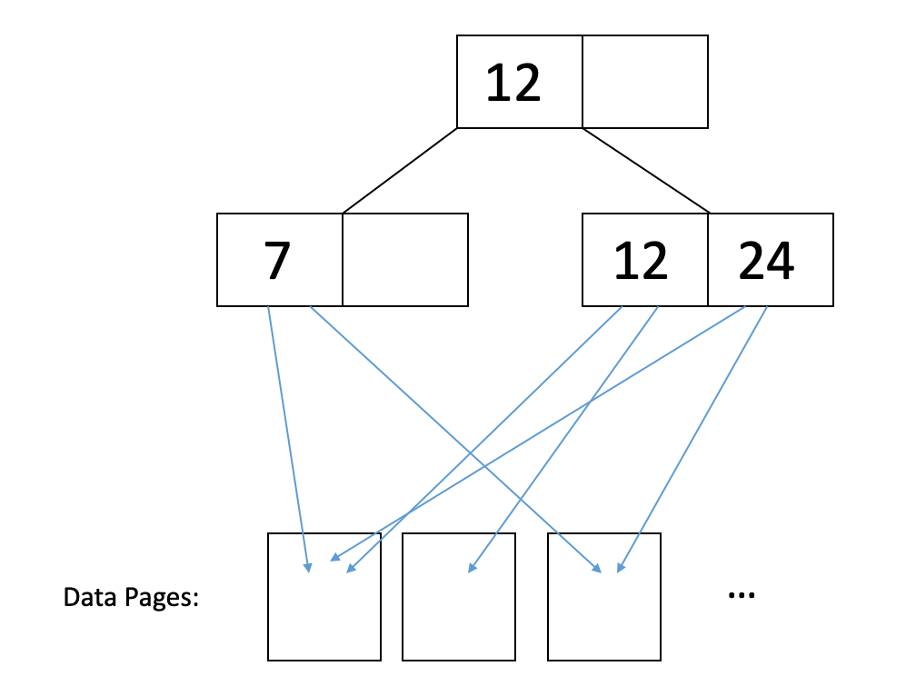
  In the figure above, if we want to read records with 12 and 24, then we would have to read in each of the data pages they point to in order to retrieve all the records associated with these keys.

• Clustered

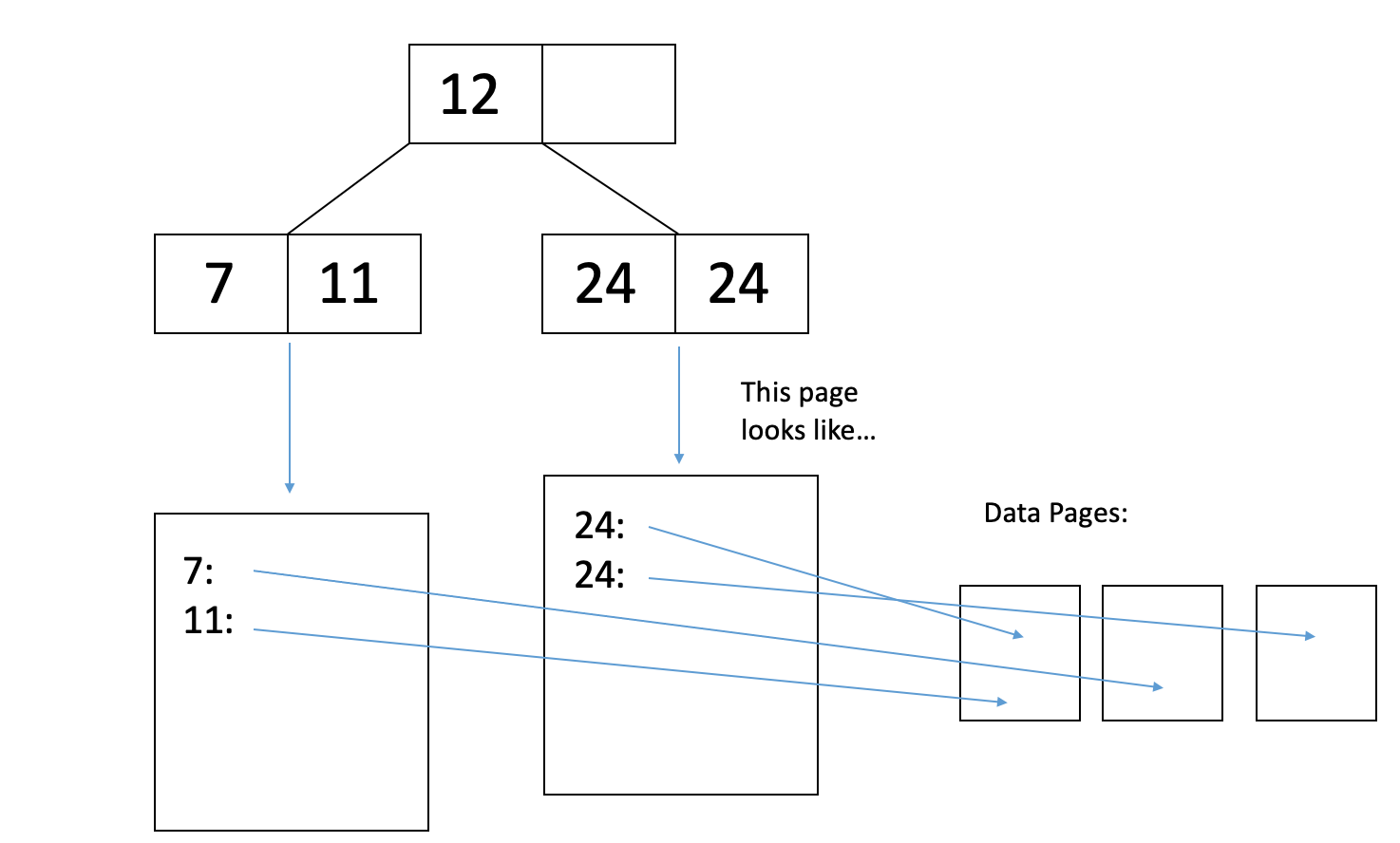
  In a clustered index, the data pages are sorted on the same index on which you’ve built your B+ tree. This does not mean that the data pages are sorted exactly, just that keys are roughly in the same order as data. The difference in I/O cost therefore comes from caching, where two records with close keys will likely be in the same page, so the second one can be read from the cached page. Thus, you typically just need to read one page to get all the records that have a common / similar key. For instance, consider this illustration:

  

  In the figure above, we can read records with 7 and 12 by reading 2 pages. If we do sequential reads of the leaf node values, the data page is largely the same. In conclusion,

• UNCLUSTERED = ~1 I/O per record.

• CLUSTERED = ~1 I/O per page of records.

• Clustered vs. Unclustered Indexes

  While clustered indexes can be more efficient for range searches and offer potential locality benefits during sequential disk access and prefetching, etc, they are usually more expensive to maintain than unclustered indexes. For example, the data file can become less clustered with more insertions coming in and, therefore, require periodical sorting of the file.

Counting IO’s

Here’s the general procedure. It’s a good thing to write on your cheat sheet:

1. Read the appropriate root-to-leaf path.

2. Read the appropriate data page(s). If we need to read multiple pages, we will allot a read IO for each page. In addition, we account for clustering for Alt. 2 or 3 (see below.)

3. Write data page, if you want to modify it. Again, if we want to do a write that spans multiple data pages, we will need to allot a write IO for each page.

4. Update index page(s).

Let’s look at an example. See the following Alternative 2 Unclustered B+ tree:

We want to delete the only 11-year-old from our database. How many I/Os will it take?

• One I/O for each of the 2 relevant index pages on the roof-to-leaf path (an index page is an inner node or a leaf node).

• One I/O to read the data page where the 11-year-old’s record is. Once it’s in memory we can delete the record from the page.

• One I/O to write the modified data page back to disk.

• Now that there are no more 11-year-olds in our database we should remove the key "11" from the leaf page of our B+ tree, which we already read in Step 1. We do so, and then it takes one I/O to write the modified leaf page to disk.

• Thus, the total cost to delete the record was 5 I/Os.

Bulk Loading

The insertion procedure we discussed before is great for making additions to an existing B+ tree. If we want to construct a B+ tree from scratch, however, we can do better. This is because if we use the insertion procedure we would have to traverse the tree each time we want to insert something new; regular insertions into random data pages also lead to poor cache efficiency and poor utilization of the leaf pages as they are typically half-empty. Instead, we will use bulkloading:

1. Sort the data on the key the index will be built on.

2. Fill leaf pages until some fill factor f. Note that fill factor only applies to leaf nodes. For inner nodes, we still follow the same rule to insert until they are full.

3. Add a pointer from parent to leaf page. If the parent overflows, we will follow a procedure similar to insertion. We will split the parent into two nodes:

   1. Keep d entries in L_1 (this means d+1 entries will go in L_2).

   2. Since a parent node overflowed, we will MOVE L_2’s first entry into the parent.

4. Adjust pointers.

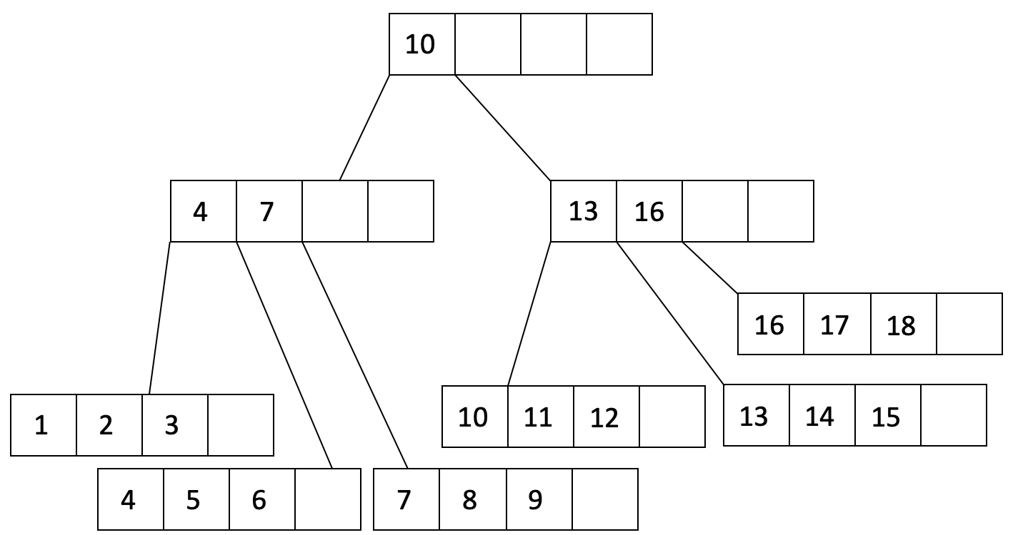
Let’s look at an example. Let’s say our fill factor is 3/4 and we want to insert 1, … , 20 into an order d=2 tree. We will start by filling a leaf page until our fill factor:

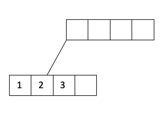
We have filled a leaf node to the fill factor of 3/4 and added a pointer from the parent node to the leaf node. Let’s continue filling:

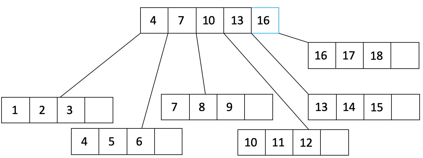
In the figure above, we see that the parent node has overflowed. We will split the parent node into two nodes and create a new parent:

As you can see from the above example, indexes built from bulkloading always start off clustered because the underlying data is sorted on the key. To maintain clustering, we can choose the fill factor depending on future insertion patterns.

Past Exam Problems

• Sp22 Quiz Q3

• Sp22 Final Q3

• Fa21 Midterm 1 Q4

• Fa21 Final Q4

• Sp21 Midterm 1 Q3

• Sp21 Final Q1

• Fa20 Midterm 1 Q4