Introduction

So far, we’ve learned how to use already built databases: SQL queries! We also learned the internals of a database management system which includes many abstraction levels. But what happens if we are given a high-level description of what data we want to store with our database? How do we design a database to fit out needs? We will discuss these question in this module!

Entity-Relationship Models

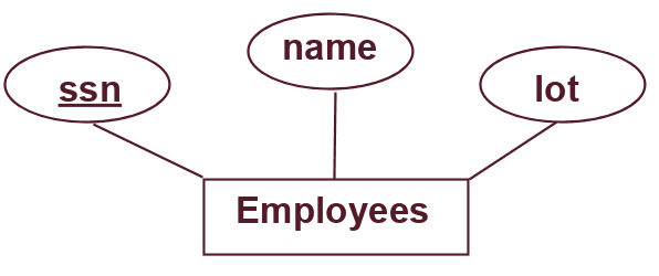
When designing a database, we often use Entity-Relationship Models (aka "E-R" models). These models have 2 main components. The first main component is an entity: a real-world object described by a set of attribute values. An entity is usually depicted as a rectangle in our E-R model. In addition, the attributes/fields associated with the entity are depicted as ovals. For example, the following figure shows an employee as an entity in our E-R model with the following fields: a SSN number, a name, and a lot. Note that the attribute "ssn" is underlined because it is the identifying attribute for this entity! In a schema, this would be the primary key.

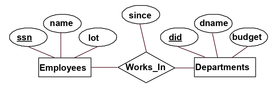
The second main component is a relationship: association among two or more entities. A relationship is usually depicted as a diamond in our E-R model. Again, the attributes associated with the relationship are depicted as ovals. For example, the following figure shows "works in" as a relationship between the entities employee and department. The "works in" relationship has the attribute "since."

Note that the same entity set can participate in different relationship sets, or in different “roles” in the same relationship set.

Relationship Constraints

We have connected our entities to relationships with a thin black line up until now. This line means denotes a many-to-many relationship. This means each entity can participate in 0 or more times in the relationship and vice versa. For example, for the figure above, this means that many employees can work in many departments (0 or more) and departments can have many employees (0 or more). In contrast, we want our model to reflect that each department has at most one manager. We do this by using a key constraint, which denotes an at most one, or 1-to-many relationship. The key constraint is depicted by a thin arrow. It is important to note the direction of the arrow, which points from the entity with 0 or 1, towards the entity with many. For example, for the following figure, this means that each department has at most one manager (0 or 1) while employees can be managers for many (0 or more) departments.

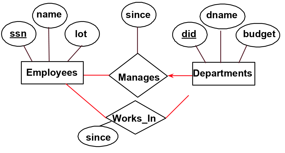
What if we want our model to show that each employee works in at least one department? We do this by using a participation constraint, which denotes at least one relationship. The participation constraint is depicted by a thick line. For example, in the following figure, we added two thick lines. One of them denotes that each employee works in at least one department. The other denotes that each department has at least one employee.

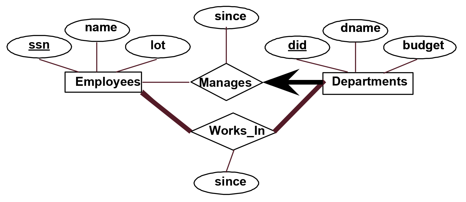
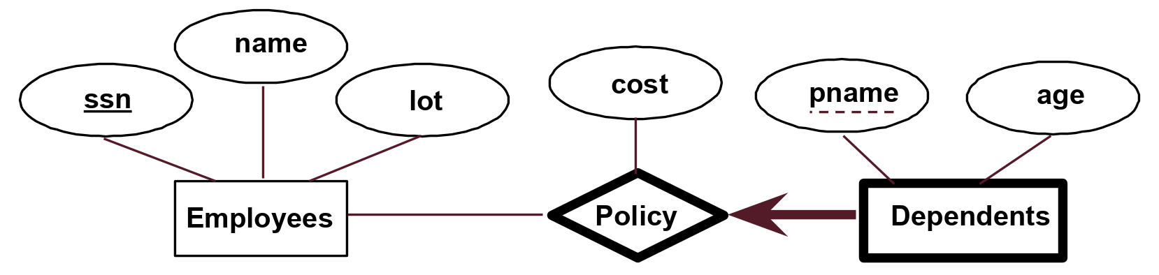
In addition, you can see we added a thick arrow pointing from departments to manages. This is both a key and participation constraint: each department has exactly one manager. A weak entity can be identified uniquely only by considering the primary key of another (owner) entity. Owner entities and weak entities must participate in a one-to-many relationship (one owner, many weak entities). The weak entity must have total participation in this identifying relationship set. We depict a weak entity by bolding the rectangle and relationship as shown below. In addition, weak entities have only a “partial key” (dashed underline). In the example below, we say that every dependent is uniquely identified by their pname and an employees’ ssn and that each employee has 0 or more dependents attached to them.

Now that we have our E-R Model drawn out, how do we actually organize it into relations? We can translate each entity and relationship to its own table and have primary keys and foreign keys depending on the relationship between tables. In general, there are many ways to set up relations to represent the same E-R model.

FDs and Normalization

Now that we have set up our database, we want to optimize! One thing we want to avoid is redundancy in our schema. This is wasted storage and also leads to insert/delete/update anomalies. Our solution to this problem is going to be Functional Dependencies. A functional dependency \(X \xrightarrow{} Y\) means that the \(X\) column determines \(Y\) column in a table \(R\). This means given any two tuples in table \(R\), if their \(X\) values are the same, then their \(Y\) values must be the same (but not vice versa). Let’s look at a couple of examples to better understand functional dependencies and what "determines" means. In the example below, two of the rows have the same X value (\(1\)) but different Y values (\(5\) and \(6\)), so we cannot say that X determines Y:

X	Y
1	5
1	6
2	1

For the following example, we see that all rows with the same X value have the same Y value. More specifically, all the rows with \(X=1\) have \(Y=2\), all the rows with \(X=2\) have \(Y=4\), and all the rows with \(X=3\) have \(Y=4\). In this case, it is possible that X determines Y (aka \(X \xrightarrow{} Y\)):

X	Y
1	2
1	2
1	2
2	4
3	4

Note that in the above example, even though \(Y=4\) for two rows, their X values do not have to be the same to say that X determines Y. We only care if the Y values for a particular X value are the same, not vice versa! Primary keys are special cases of FDs. A superkey¹ is a set of columns that determine all the columns in the table. If \(X\) is a superkey of table \(R\), then \(X \xrightarrow[]{} R\).

A candidate key is a set of columns that determine all the columns in the table such that if we remove any of the columns in a candidate key, the resulting set will not be a superkey of the relation. You can think of it as the minimum set of columns that is a superkey for the table. If \(X\) is a candidate key of \(R\), then \(X \xrightarrow[]{} R\) and for every strict subset \(Y \subset X\), \(Y \nrightarrow{} R\).

For example, if columns \(K, L\) are the columns in a table and \(K\) is a primary key of the table (aka column \(K\) alone determines all the columns in the table) then \(KL\) is superkey and \(K\) is a superkey and a candidate key.
We will decompose our relation to avoid redundancies by using functional dependencies. But first, we define the closure of \(F\), denoted as \(F+\), to be the set of all FDs that are implied by \(F\). In broader terms, a closure is the full set of table relationships that can be determined from known FDs.

Let’s take a look at a couple of examples to better understand these definitions. Given a relation \(R\) with columns \(\{A,B,C,D,E\}\) and functional dependencies \(F=\{B \xrightarrow{} CD, D \xrightarrow{} E, B \xrightarrow{} A, E \xrightarrow{} C, AD \xrightarrow{} B\}\), let’s examine the following questions:

Is \(B \xrightarrow{} E\) in \(F+\)? Yes! To see why, we will evaluate the closure of \(B\). \(B+ = \{ B, C, D, E, A\}\), we get this because \(B\) determines \(CD\) from the first functional dependency from the set \(F\). Then we see that \(D\) determines \(E\) so \(E\) is in the closure of \(B\). Thus, from the given implications in F, we see that \(B \xrightarrow{} E\), so the answer is YES.
Is \(D\) a superkey for relation \(R\)? We will determine the answer to this by evaluating the closure of \(D\). \(D+ = \{ D, E, C\}\). We get this because \(D\) determines itself. From the second FD in \(F\), we see that \(D\) determines \(E\). Then we see that \(E\) determines \(C\). Since \(D+\) is not equal to all the columns of the relation \(R\), we know that \(D\) is NOT a superkey for \(R\) because knowing \(D\) does not determine all columns in \(R\). The answer is NO.
Is \(AD\) a superkey for \(R\)? We again evaluate the closure of \(AD+\). Using the same procedure as the last two, we get that \(AD+ = \{ A,D,E,C,B\}\). Therefore, the answer is YES.
Is \(AD\) a candidate key for \(R\)? We must see if \(AD\) is the minimum subset to imply \(R\) by checking the closure of each subset. So we check \(A+ = \{A\}\) and \(D+ = \{ D,E,C\}\). Since none of them are \(R\) and that they together make up all columns of \(R\), we know that \(AD\) is a candidate key! The answer is YES.
Is \(ADE\) a candidate key for \(R\)? We know that \(AD\) determines all the columns for \(R\) already so \(ADE\) is NOT a candidate key. The answer is NO.

BCNF Decomposition

We will now decompose the relation into Boyce-Codd Normal Form (BCNF). Relation \(R\) with FDs \(F\) is in BCNF if for all \(X \xrightarrow{} A\) in \(F+\), either of the following conditions holds true:

\(A \subseteq X\) (called a trivial FD)
\(X\) is a superkey for \(R\) (implies \(X+ = R)\)

The BCNF Decomposition algorithm is as follows:

Input R: Relation
Input F: FDs for R
\[R = \{R\}\]
If there is a relation \(r \in R\) that is not BCNF and has \(> 2\) attributes (note that two attribute relations are always in BCNF):
1. Pick a violating FD \(f\): \(X \xrightarrow{} A\) such that \(X, A \in\) attributes of \(r\).
2. Compute \(X+\).
3. Let \(R_1 = X+\). Let \(R_2 = X \ \cup \ (r - X+)\).
4. Remove \(r\) from \(R\).
5. Insert \(R_1\) and \(R_2\) into \(R\).
6. Recompute \(F\) as FDs over all relations \(r \in R\).
Repeat step 4 until necessary.

Once these steps are completed, our relation is in Boyce-Codd Normal Form.

Let’s take a look at an example to see how this works. Let us look at relation \(R = \{C,S,J,D,P,Q,V \}\) with the superkey \(C\) and \(F = \{ JP \xrightarrow{} C, SD \xrightarrow{} P, J \xrightarrow{} S\}\).

\(JP \xrightarrow{} C\) does not violate the BCNF constraints, since \(C\) is a superkey, therefore \(JP\) is also a superkey.
The FD \(SD \xrightarrow{} P\) is in violation of BCNF since \(SD\) is not a superkey nor is \(P \subseteq SD\).
- Compute \(SD+ = \{S, D, P\}\).
- Decompose \(R\) into \(R_1 = SD+ = \{S, D, P\}\) and \(R_2 = SD \ \cup \ (R - SD+) = \{S, D\} \ \cup \{C, J, Q, V\} = \{S, D, C, J, Q, V\}\).
- We now have 2 relations: \(R_1 = \{S, D, P\}\) and \(R_2 = \{S, D, C, J, Q, V\}\).
The FD \(J \xrightarrow{} S\) is in violation of BCNF since \(J\) is not a superkey for \(R_2\) nor is \(S \subseteq J\). \(R_1\) does not have this dependency so it is not decomposed further. Applying the same steps as above we see that \(R_2\) gets decomposed into \(\{J, S\}\) and \(\{D, C, J, Q, V\}\).

The BCNF form of this relation is \(SDP\), \(JS\), and \(DCJQV\).

Lossless Decomposition

One problem that can arise from decomposing relations is that after breaking up the table into smaller relations, we may be unable to reconstruct the original relation through these decomposed relations. This means that our decomposition is lossy.

For example, consider the following relation R=ABC, which is decomposed into X=AB and Y=BC. This is a lossy decomposition since attempting to reconstruct R by joining X and Y doesn’t give us the original relation, but rather a superset of R with some extra junk data. As we can see in this example, lossy decompositions don’t "lose" data, but rather generate bad data.\

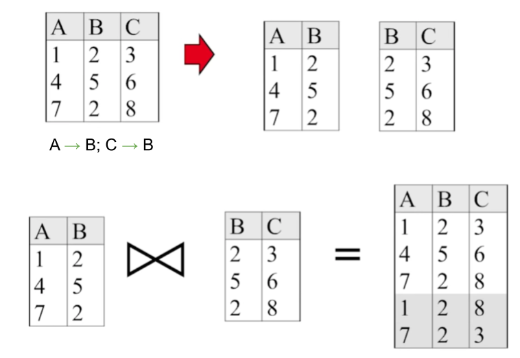
Instead, we want our decompositions to be lossless, meaning that if R is decomposed into X and Y, \(X \bowtie Y = R\). A decomposition of a relation R into X and Y is lossless with respect to F (a set of FDs) if and only if the closure of F (\(F^+\)) contains:

\(X \cap Y \xrightarrow[]{} X\) (\(X \cap Y\) is a superkey of X), or
\(X \cap Y \xrightarrow[]{} Y\) (\(X \cap Y\) is a superkey of Y)

Looking back at our previous example (R = ABC, X=AB, Y=BC), we can apply this test to confirm it is lossy. \(X \cap Y = B\) , and B is not a superkey of either X or Y (because in X, B = 2 maps to two different values for A; in Y, B = 2 maps to two different values for C).

BCNF decompositions are always lossless, so we don’t have to worry about lossiness if we are decomposing a relation into BCNF.

Dependency Preserving Decompositions

Another problem that can arise from decomposing relations is that dependency checking may require joins. If we make an insertion to a table and need to check that functional dependencies are still satisfied, we may have to join together the tables we decomposed, making every insertion we do costly.

We can avoid this problem through dependency preserving decompositions. Suppose we decompose R into X, Y, and Z. This decomposition is dependency preserving if enforcing FDs individually on each of X, Y, and Z implies that all FDs that held on R must also hold. Now, when making an insertion to a table, we will only need to check the FDs are satisfied on that relation (avoiding joins between decomposed relations) since this will be sufficient for enforcing all FDs that held on the original relation.

Formally, a decomposition of a relation R into X and Y is dependency preserving if \((F_X \cup F_Y)^+ = F^+\). If we take the dependencies that can be checked in X without considering Y and the dependencies that can be checked in Y without considering X, the closure of their union will be the closure of the original set of FDs (\(F^+\)).

Note that although decompositions into BCNF are lossless, they are not necessarily dependency preserving! To demonstrate this, let’s revisit the BCNF decomposition example we examined earlier, where the relation \(R = \{C,S,J,D,P,Q,V \}\) with the superkey \(C\) and \(F = \{ JP \xrightarrow{} C, SD \xrightarrow{} P, J \xrightarrow{} S\}\) was decomposed into X = \(SDP\), Y = \(JS\), and Z = \(DCJQV\).

Here, \(F_X = \{SD \xrightarrow{} P\}\), \(F_Y = \{J \xrightarrow{} S\}\), and \(F_Z = \{\}\). Thus, \((F_X \cup F_Y \cup F_Z) = \{SD \xrightarrow{} P, J \xrightarrow{} S\}\), and the closure of this set of FDs does not include \(JP \xrightarrow{} C\). Thus, this BCNF decomposition is not dependency preserving.

Practice Questions

Consider a set of functional dependencies F = {X \(\rightarrow{}\) Y, Y \(\rightarrow{}\) Z}. For each of the following symbols or expressions, indicate whether it is (a) an attribute, (b) a set of attributes, (c), a set of sets of attributes, (d) a functional dependency, (e) a set of functional dependencies, or (f) none of the above.
1. X
2. XY
3. X \(\rightarrow{}\) Y
4. F
5. F+
6. X+
7. Armstrong’s reflexivity axiom
Let’s say we have two entities, Students and School, connected by the relationship "Attend s". If a student can attend at most one school, but does not have to attend, what kind of line would we want from Students to Attends?
From the previous question, we also know that each school has at least one student. What kind of line would we want from School to Attends?
Instead, we decide to keep the Student entity but replace school with a Semester entity and connect them with the relationship "Enrolled". A student can be enrolled for up to 10 semesters. What kind of line would we want from Students to Enrolled?
We know that D and AB are both superkeys of the table R. Can both of them also be candidate keys? Are they both guaranteed to be candidate keys?
Decompose ABCDEFGH into BCNF in the order of the following FDs: \(\{G \xrightarrow{} H, EF \xrightarrow{} B, EA \xrightarrow{} C, FH \xrightarrow{} D\}\)
Decompose ABCDEF into BCNF in the order of the following FDs: \(\{A \xrightarrow{} B, B \xrightarrow{} CD, DE \xrightarrow{} F, D \xrightarrow{} A\}\)
Is the decomposition in #6 lossless? Is it dependency preserving?
Suppose we have a relation "tv_shows". Suppose we also have a relation "awards". The awards entity is also a weak entity connected to the tv_shows entity through a "won" relationship. What kind of edge will be drawn between the won relationship and the awards entity set?

Solutions

Consider a set of functional dependencies F = {X \(\rightarrow{}\) Y, Y \(\rightarrow{}\) Z}. For each of the following symbols or expressions, indicate whether it is (a) an attribute, (b) a set of attributes, (c), a set of sets of attributes, (d) a functional dependency, (e) a set of functional dependencies, or (f) none of the above.
1. X [(b) a set of attributes (or a set of columns)]{style=”color: red”}
2. XY [(b) a set of attributes]{style=”color: red”}
3. X \(\rightarrow{}\) Y [(d) a functional dependency]{style=”color: red”}
4. F [(e) a set of functional dependencies]{style=”color: red”}
5. F+ [(e) a set of functional dependencies]{style=”color: red”}
6. X+ [(b) a set of attributes]{style=”color: red”}
7. Armstrong’s reflexivity axiom [(f) an axiom]{style=”color: red”}
We know a student can attend at most one school, so the line between Students and Attends should be a thin arrow.
We know each school has at least one student, so the line between School and Attends should be a thick line.
We know a student can be enrolled for 0 or more semesters, so the line between Students and Enrolled should be a thin line.
Both D and AB are possible candidate keys. AB is a possible candidate key if removing A or B causes it to no longer be a superkey. Only D is guaranteed to be a candidate key. This is because there is nothing we can remove from the set of columns and possibly have a smaller set that is a superkey because D is only one column. On the other hand, AB is not guaranteed to be a candidate key because removing A or B might result in a smaller set that is still a superkey.
At step 1, we get ABCDEFG and GH.

At step 2, we get ACDEFG and EFB and GH.

At step 3, we get ADEFG and EAC and EFB and GH.
First, we consider \(A \rightarrow{} B\). A+ = ABCD so we get ABCD and AEF.

Next, we consider \(B \rightarrow{} CD\). Since B is a superkey (B+ = ABCD), BCNF is not violated and we do not need to decompose.

Next, we consider \(DE \rightarrow{} F\). We do not need to decompose as there are no relations with D, E, and F in them.

Next, we consider \(D \rightarrow{} A\). Since D is a superkey (D+ = ABCD), BCNF is not violated and we do not need to decompose.
In #6, we split R = ABCDEF into X = ABCD and Y = AEF. This decomposition is lossless, as all BCNF decompositions are lossless. We can confirm this by noticing that \(X \cap Y = A\), and A is a superkey of X.

However, this decomposition is not dependency preserving. \(F_X = \{ A \rightarrow{} B, B \rightarrow{} CD, D \rightarrow{} A\}\) and \(F_Y = \{\}\). \((F_X \cup F_Y)^+\) does not contain \(DE \rightarrow{} F\), an FD that originally held on R.
Since "awards" is a weak entity, we will draw a bolded arrow from "awards" to "won". We will also bold the "awards" rectangle and "won" diamond.

Past Exam Problems

Fa22 Midterm 2 Q3
Fa22 Midterm 2 Q4
Sp22 Final Q11
Fa21 Midterm 2 Q1
Sp21 Midterm 2 Q1
Fa20 Final Q5

Sometimes we refer to a superkey as a key. ↩