Spatial and Vector Indexes

So far our focus has been on 1 dimensional indices. In the previous note we explored B+ trees where the search key is a single integer or string. Now we will explore search on multi-column keys. In this note we introduce the Spatial Index: A type of index that allows you index multiple columns at once, often by treating pairs of values as coordinates in the cartesian plane. Spatial indices are also used to index data that naturally occurs in pairs (e.g. latitudes and longitudes, points in multidimensional space, etc). For this class, we will examine the basics of spatial indices and discuss the implementation of them through the KD Tree.

Motivation

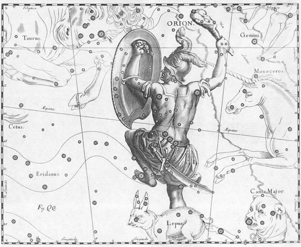
Astronomy

Suppose we have a map of the stars with their x,y coordinates. We want to answer each of the following questions:

1. Does a given (x, y) coordinate contain a star?
   Equality Search

2. How many stars are in a region of the map? A region is a area of the map bounded by 4 coordinates.
   Range Search

3. What are the stars closest to a given (x,y) coordinate?
   Nearest Neighbor

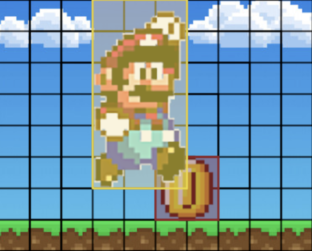
Graphics

Suppose we are coding a game with characters and items represented as objects on the screen. We want to answer the following questions about the display:

1. Do any two objects touch each other? In other words, are two objects located at the same (x, y) coordinate?
   Equality Search

2. How many objects should be rendered within the boundaries of the screen?
   Range Search

In these examples, it is often inefficient and expensive to try to solve these problems with a 1 dimensional index like the B+ Tree. Thus, we introduce the K-D tree!

K-D Tree

By definition, a KD Tree is a space-partitioning data structure used to organize points in a k-dimensional space. The general idea is to build a balanced binary tree that splits on multiple dimensions. Compare this to the B+ tree, which only splits on one dimension.

Why would we do this?
The goal is to enable fast look up, range queries, and nearest neighbor search on multiple dimensions.

For simplicity we will use 2-D points to illustrate a K-D tree, but in general we can use any number of dimensions (hence the “k” in K-D).

Tree Construction

The general procedure for creating a K-D tree is below:

1. If we have a single point, then the point forms the tree.
2. Otherwise, divide the points in half by a line perpendicular to one of the axes.
3. Recursively construct k-d trees for the two partitioned sets of points.

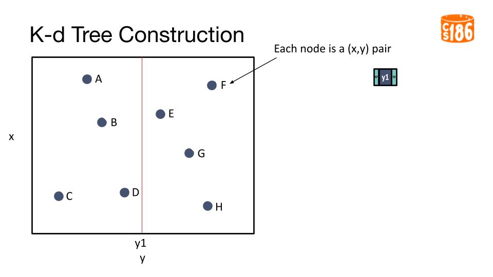
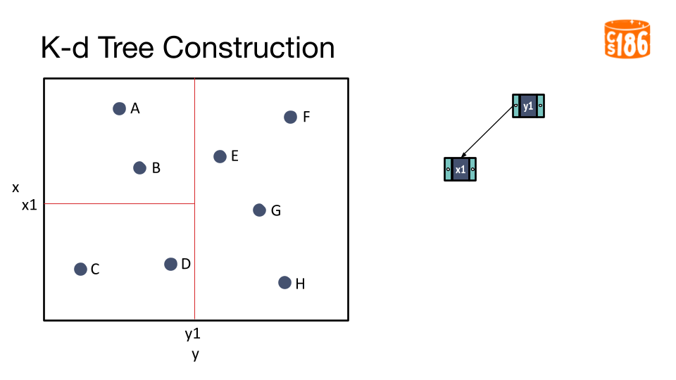
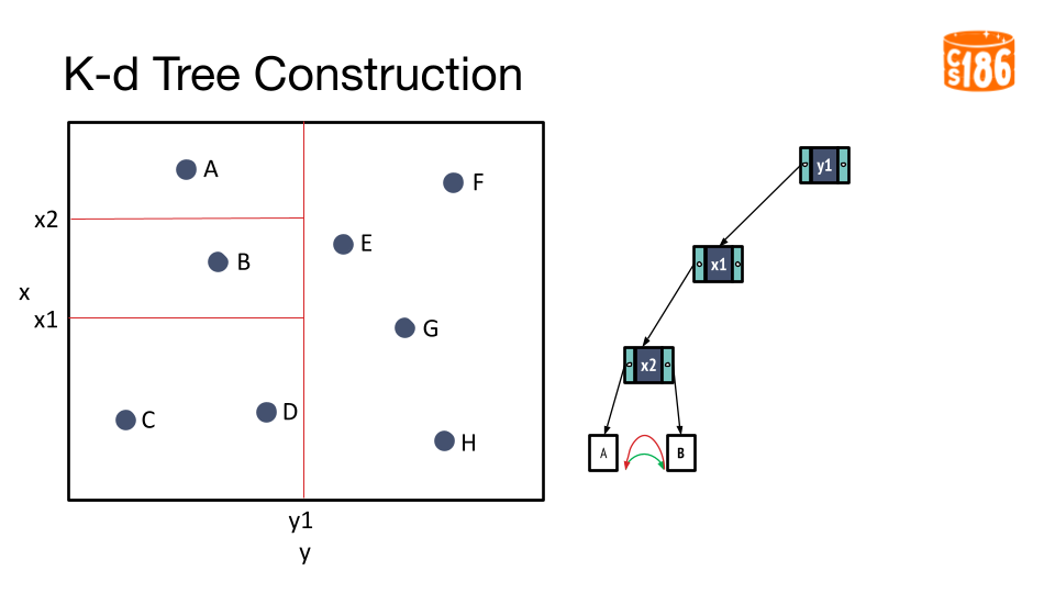
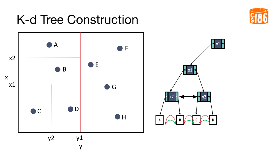
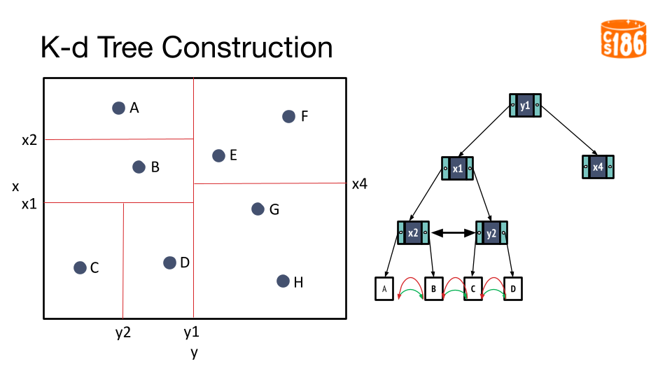
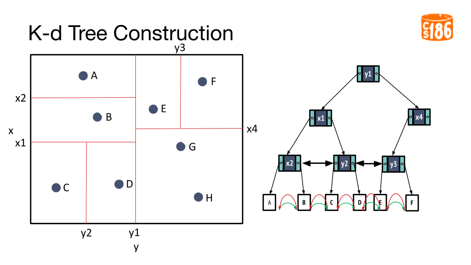
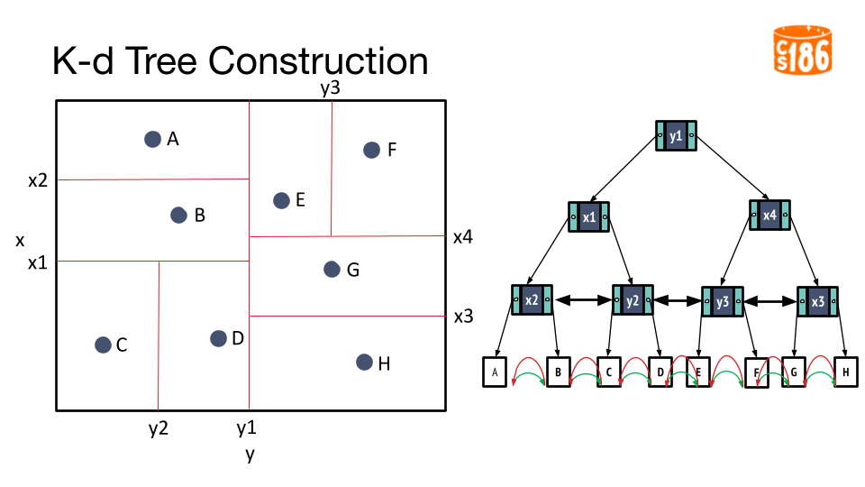
But how do we divide the points?

• We could divide in a round-robin fashion across two dimensions
• We could divide on the median value on one of the dimensions.

(Optional) Other Choices for splitting a K-D Tree.

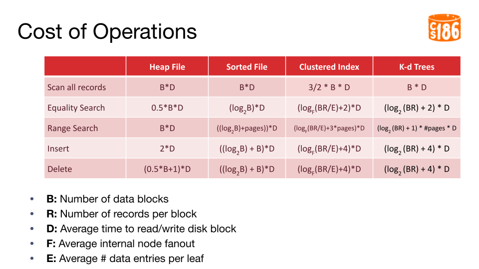
Cost of Operations

For the rest of this note, we will use the following variables to represent the cost of each operation in I/Os.

• B: Number of data blocks
• R: Number of records per block
• D: Average time to read/write disk block
• F: Average internal node fanout
• E: Average # data entries per leaf

Equality Search

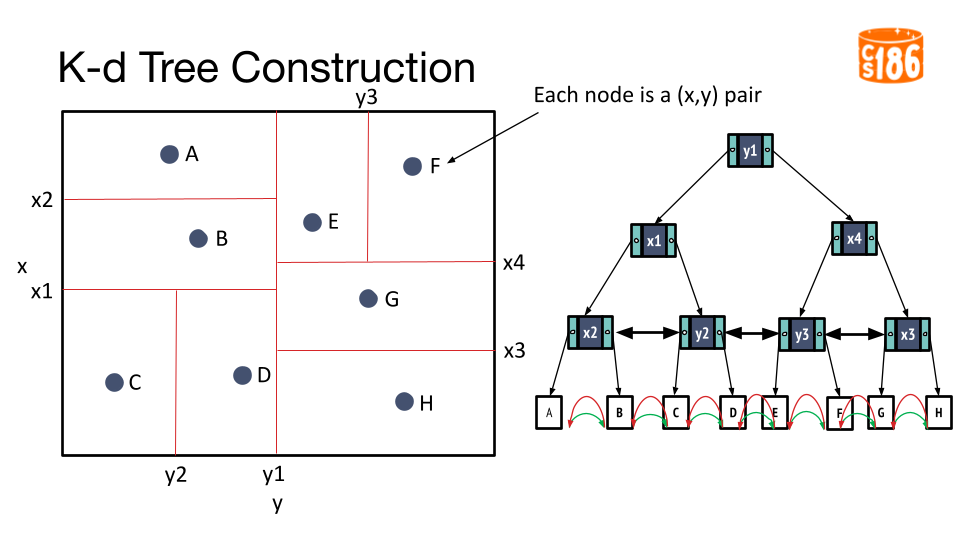
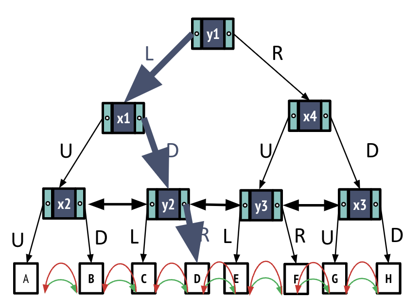
Assume there exists a node D in the K-D Tree. Since we are working in 2 dimensions, node D has an x value D.x and a y value D.y. Our goal is to find node D in the tree (i.e. an equality search).

1. Start from the root node.
2. Compare D.y with y1. We see that D.y is less than y1.
3. Follow pointer to the left subtree
4. Compare d.x with x1. Assume we we see that D.x is greater than x1.
5. Follow the pointer to the right subtree
6. Recursively repeat process until we reach the leaf node.

I/O Cost: log(BR)

Range search

Now assume we are interested in a range of points in our K-D Tree. We can use the following algorithm for range search:

1. Search index to find first page to read
2. Scan the leaf pages to find which heap pages to read
3. Read the corresponding heap pages

• I/Os for 1: log(BR) + 1
  Note we have +1 for the index leaf page
• I/Os for 3: #pages
  #pages: number of pages storing records that matches search criteria
• I/Os for 2: #pages
  over-approximate and assume same as 3

I/O Cost: (log(BR) + 1 + (2 * #pages)) * D

Insertion

Now assume we want to insert a new entry into our database (and as a result a new node into the K-D tree).

1. Search index to find heap file page to modify
2. Read corresponding page and modify in memory
3. Write back the modified index leaf and heap file pages

• I/Os for 1: log(BR) + 1
• I/Os for 2: 1
• I/Os for 3: 2

Total cost : (log(BR) + 4) * D

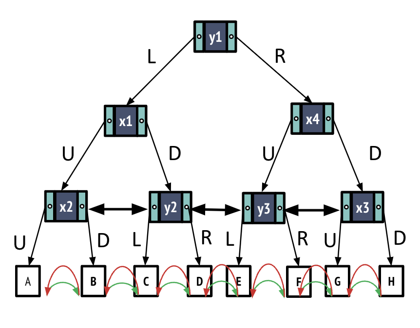
Table of I/O Costs

Nearest neighbor search

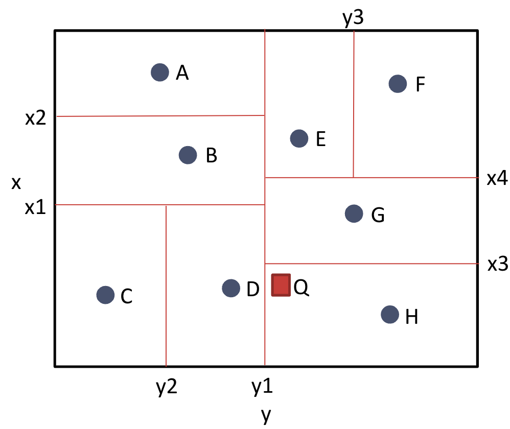
The previous operations are all ones we’ve seen before with B+ Trees. The K-D tree allows us to perform another type of search that is incredibly useful in computer science. Nearest Neighbor Search is the search algorithm used to find the closest point in a K-D tree to a given input. For instance in the following example, we provide input Q and would expect the N-N algorithm to return the point closest to Q (closest defined by Euclidean distance). In this case, that would be D.

General Idea: Traverse down the tree and keep track of the closest point found so far. Stop when we know that there can’t be any other point closer.

• Number of traversals is proportional to log(nodes)
• Stop when we know that there can’t be a closer point in the tree
• Traverse all nodes in the worst case

We can generalize this algorithm to find N-nearest neighbors (but won’t prove that here).

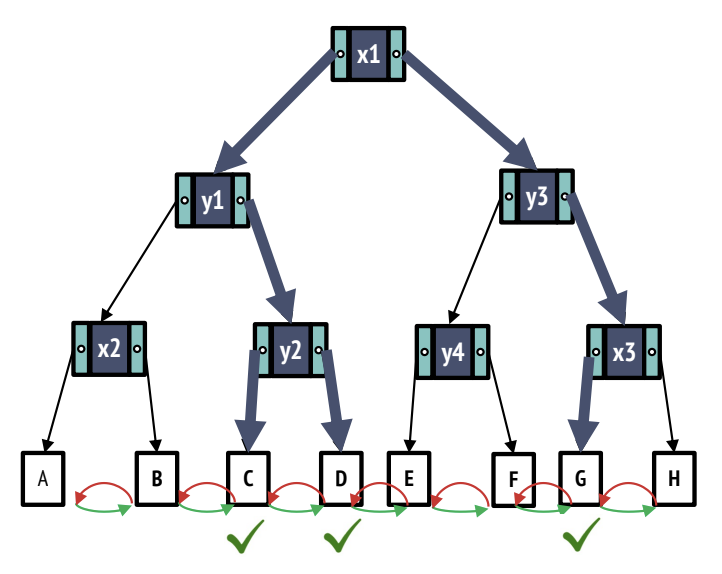
Nearest Neighbor Example

Let’s walk through the example from before to find the closest point for Q. Note that the tree for the example above is below.

1. Q is right of y1, so we go right from the root.
2. Q is below x4, so we go down.
3. Q is below x3, so we go down. This is the first time we encounter a point, so we mark that H is the closest point we’ve seen so far.
4. Go back up to x3 and now go up (the other branch). The leaf node is G, which is closer than H so G is our closest point.
5. Now we go back up to x4, and traverse the other branch (go up).
6. Q is less than y3 so we go Left. The leaf node is E, which is farther than G. We know anything in the region of the other branch (right from y3 will be) farther than our best choice so far, so we can skip that branch and continue our algorithm. How do we know anything in that region will be farther than our best choice? Well, we know the boundaries of that region, so we can compute the euclidean distance to the closest point in that region (i.e. The corner closest to Q) which is farther than our current best. Thus, anything in that region is farther than our nearest neighbor so far.
7. Now we can go back up to the root and go left this time.
8. Q is down of x1, so we go down.
9. Q is right of y2 so we go right to reach the node D. Now our closest node is D. Using the logic from step 6, we can eliminate the rest of the possible branches (because we’ve found the actual closest neighbor).

Conclusion

In the examples in this note, we only worked with K-D trees of 2 dimensions. In general though, K-D trees can be extended to even higher dimensions. Some variations: R-tree, Quadtree, Octree. The primary application of this structure has been finding nearest neighbors, which is supported by Postgres, Oracle, SQLServer. Being able to efficiently find the nearest neighbors for a given data point can be extremely useful when working on recommendation systems and image recognition.