Motivation
Sometimes, sorting is a bit overkill for the problem. Often, all we want is to group the same value together, but we do not actually care about the order the values appear in (think GROUP BY or de-duplication). In a database, grouping like values together is called hashing. We cannot build a hash table in the standard way you learned in 61B for the same reason we could not use quick sort in the last note: we cannot fit all of our data in memory! Let’s see how to build an efficient out-of-core hashing algorithm.
General Strategy
Because we cannot fit all of the data in memory at once, we’ll need to build several different hash tables and concatenate them together. There is a problem with this idea though. What happens if we build two separate hash tables that each have the same value in them (e.g. “Brian” occurs in both tables)? Concatenating the the tables will result in some of the “Brian”s not being right next to each other.
To fix this, before building a hash table out of the data in memory, we need to guarantee that if a certain value is in memory, all of its occurrences are also in memory. In other words, if “Brian” occurs in memory at least once, then we can only build the hash table if every occurrence of “Brian” in our data is currently in memory. This ensures that values can only appear in one hash table, making the hash tables safe to concatenate.
The Algorithm
We will use a divide and conquer algorithm to solve this problem. During the “divide” phase we perform partitioning passes, and during the “conquer” phase we construct the hash tables. Just like in the sorting note, we will assume that we have \(B\) buffer frames available to us. As we hash our data, we will use \(1\) of these buffers as an input buffer, and \(B-1\) of these buffers as output buffers.
We begin by streaming data from disk into our \(1\) input buffer. Once we have the input data, we want to break it into partitions. A partition is a set of pages such that for a particular hash function, the values on the pages all hash to the same hash value. The first partitioning pass will hash each record in the input buffer into one of \(B-1\) partitions, with each partition corresponding to one of our \(B-1\) output buffers. If an output buffer fills up, that page is flushed to disk, and the hashing process continues. Any flushed pages that came from the same buffer will be located adjacent to each other on disk. At the end of the first partitioning pass, we have \(B-1\) partitions stored on disk, with each partition’s data stored continuously.
One important property of partitions is that if a certain value appears in one partition, all occurrences of that value in our data will be located in the same partition. This is because identical values will be hashed to the same value. For example, if “Brian” appears in one partition, “Brian” will not appear in any other partition.
After the first partitioning pass, we have \(B-1\) partitions of varying sizes. For partitions that can fit in memory (the partition’s size is less than or equal to \(B\) pages), we can go right into the “conquer” phase, and begin building hash tables. For the partitions that are too big, we need to recursively partition them using a different hash function than we used in the first pass. Why a different hash function? If we reused the original function, every value would hash to its original partition so the partitions would not get any smaller. We can recursively partition with different hash functions as many times as necessary until all of the partitions have at most B pages.
Once all of our partitions can fit in memory, and all of the same values occur in the same partition (by the property of partitions), we can begin the the “conquer” phase. First we select a new hash function for the purpose of building our final hash table. Then, for each partition, we stream the partition into memory, create a hash table using the new hash function, and flush the resulting hash table back to disk.
Drawbacks of Hashing
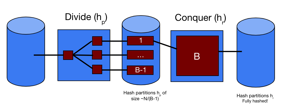
It is important to note that hashing is very susceptible to data skew. Data skew occurs when the values that we are hashing do not follow a uniform distribution. Due to the property of hashed partitions (that all hashes of the same value will end up in the same partition), data skew can lead to very unevenly-sized partitions, which is sub-optimal for our purposes. Additionally, not all hash functions are created equal. In the optimal case, our hash function is a uniform hash function, which partitions the data into "uniform", equal-sized partitions. However, hash functions are often non-uniform, and partition data unevenly across all of the partitions. For the purposes of this class, we will be using uniform hash functions unless otherwise stated. In the two images below, cylinders represent steps that happen on disk, squares represent steps that happen in memory, and the lines between the two represent data streaming from disk to memory and vice versa.
The image below shows the two phases of Hashing - divide and conquer - when recursive partitioning isn’t required. This means that after initial partitioning, all partitions fit within \(B\) pages. Notice that in the Divide phase, \(1\) buffer page is dedicated to the input buffer and the remaining \(B-1\) are used for partitioning. Afterwards, in the Conquer phase, a separate hash function \(h_r\) is used on each individual partition to form in-memory hash tables.
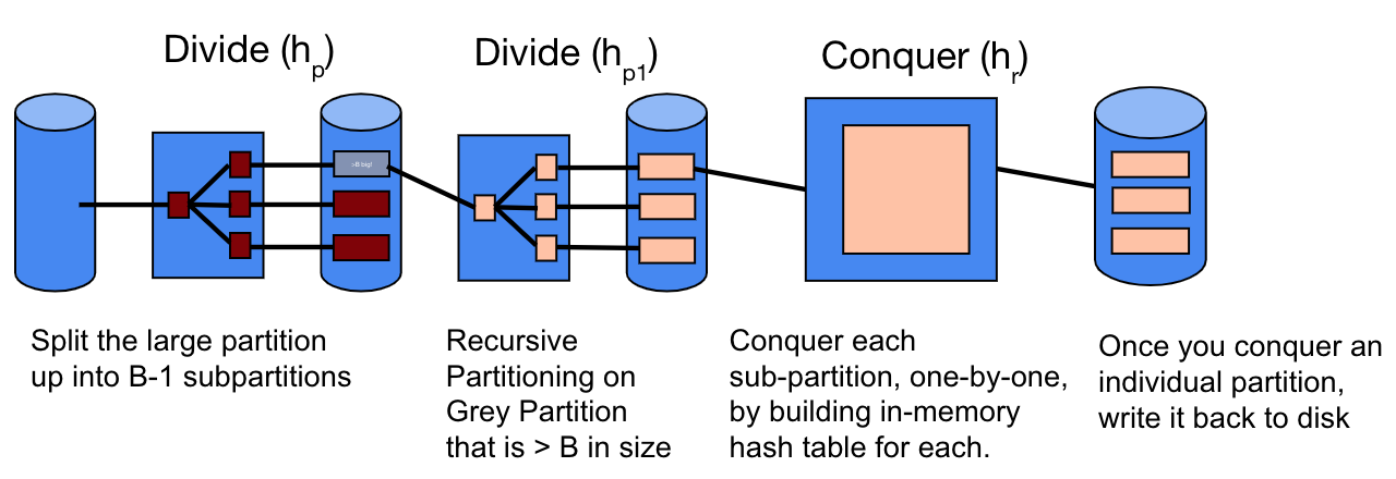
The image below shows recursive partitioning. Notice that the additional phases only apply to the partition with size greater than \(B\) pages (grey partition).
Example
In the following example, we will assume that we have \(B=3\) buffer pages available to us. We also assume that Brian and Eric hash to the same value for the first hash function but different values for the second hash function, and Jamie and Lakshya hash to the same value for the first hash function.
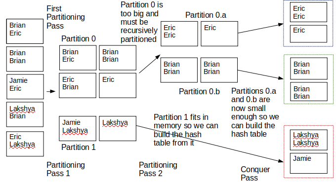
After the first partitioning pass (Partitioning Pass 1), Partition 0 is 4 pages, and Partition 1 is 2 pages. Partition 1 fits in memory, but Partition 0 does not. This means we must recursively partition Partition
- After Partitioning Pass 2, Partition 0 is broken into two parts: Partition 0.a is 2 pages, and Partition 0.b is 2 pages. As Partition 1 already fit into memory, it was not partitioned during Partitioning Pass
- Once all partitions (0.a, 0.b, 1) fit into memory, we perform the Conquer Pass and build the hash tables. You can see that after the final Conquer Pass, all of the like values are next to each other, which is our end goal.
Analysis of External Hashing
We’re not going to be able to create a simple formula to count the number of I/Os like in the sorting algorithm because we do not know how large the partitions will be. One of the first things we need to recognize is that it is possible for the number of pages in the table to increase after a partitioning pass. To see why, consider the following table in which we can fit two integers on a page:
[1, 2] [1, 4] [3, 4]
Let’s assume B=3, so we only divide the data into 2 partitions. Let’s assume 1 and 3 hash to partition 1, and 2 and 4 hash to partition 2. After partitioning, partition 1 will have:
[1, 1], [3]
And partition 2 will have:
[4, 2], [4]
Notice that we now have 4 pages when we only started with 3. Therefore, the only reliable way to count the number of I/Os is to go through each pass and see exactly what will be read and what will be written. Let \(m\) be the total number of partitioning passes required, let \(r_i\) be the number of pages you need to read in for partitioning pass \(i\), let \(w_i\) be the number of pages you need to write out of partitioning pass \(i\), and let \(X\) be the total number of pages we have after partitioning that we need to build our hash tables out of. Here is a formula for the number of I/Os:
\[(\sum_{i=1}^m r_i + w_i) + 2X\]The summation doesn’t tell us anything that we didn’t already know; we need to go through each pass and figure out exactly what was read and written. The final \(2X\) part, says that in order to build our hash tables, we need to read and write every page that we have after the partitioning passes.
Here are some important properties:
- \[r_0 = N\]
- \[r_i \le w_i\]
- \[w_i \ge r_{i+1}\]
- \[X \ge N\]
Property 1 says that we must read in every page during the first partitioning pass. This comes straight from the algorithm.
Property 2 says that during a partitioning pass we will write out at least as many pages as we read in. This comes directly from the explanation above - we may create additional pages during a partitioning pass.
Property 3 says that we will not read in more pages than what we wrote out during the partitioning pass before. In the worst case, every partition from pass \(i\) will need to be repartitioned, so this would require us to read in every page. In most cases, however, some partitions will be small enough to fit in memory, so we can read in fewer pages than we produced during the previous pass.
Property 4 says that the number of pages we will build our hash table out of is at least as big as the number of data pages we started with. This comes from the fact that the partitioning passes can only increase the number of data pages, not decrease them.
Practice Questions
1) How many IOs does it take to hash a 500 page table with B = 10 buffer pages? Assume that we use perfect hash functions that distribute values evenly across all partitions.
2) We want to hash a 30 page table using B=6 buffer pages. Assume that during the first partitioning pass, 1 partition will get 10 data pages and the rest of the pages will be divided evenly among the other partitions. Also assume that the hash function(s) we use for recursive partitioning are perfect. How many IOs does it take to hash this table?
3) If we had 20 buffer pages to externally hash elements, what is the minimum number of pages we could externally hash to guarantee that we would have to use recursive partitioning?
4) If we have B buffer pages, and the table is \(B^2\) pages large, how many passes do we need to hash the table? Assume that we use perfect hash functions.
5) If we have 10 buffer pages, what is the minimum size of the table in pages, such that it needs at least two partitioning passes when hashing (i.e. at least three passes over the data)?
Solutions
1) The first partitioning pass divides the 500 pages into 9 partitions. This means that each partition will have 500 / 9 = 55.6 \(\implies\) 56 pages of data since we round up to full pages. We had to read in the 500 original pages, but we have to write out a total of 56 * 9 = 504 because each partition has 56 pages and there are 9 partitions. The total number of IOs for this pass is therefore 500 + 504 = 1004.
We cannot fit any partition into memory because they all have 56 pages, so we need to recursively partition all of them. On the next partitioning pass each partition will be divided into 9 new partitions (so 9*9 = 81 total partitions) with 56 / 9 = 6.22 \(\implies\) 7 pages each. This pass needed to read in the 504 pages from the previous pass and write out 81 * 7 = 567 pages for a total of 1071 IOs.
Now each partition is small enough to fit into memory. The final conquer pass will read in each partition from the previous pass and write it back out to build the hash table. This means every page from the previous pass is read and written once for a total of 567 + 567 = 1134 IOs.
Adding up the IOs from each pass gives a total of 1004 + 1071 + 1134 = 3209 IOs
2) There will be 5 partitions in total (B-1). The first partition gets 10 pages, so the other 20 will be divided over the other 4 partitions, meaning each of those partitions gets 5 buffer pages. We had to read in all 30 pages to partition them, and we write out 5 * 4 + 10 = 30 pages as well, meaning the first partitioning pass takes 60 IOs.
The partitions that are 5 pages do not need to be recursively partitioned because they fit in memory. The partition that is 10 pages long, however, does. This partition will be repartitioned into 5 new partitions of size 10/5 = 2 pages. We read in all 10 pages for this partition, and we wrote out 5 * 2 = 10 pages, meaning that this recursive partitioning pass takes 20 IOs.
The final conquer pass needs to read in and write out every partition, so it will take 4 * 5 * 2 = 40 IOs to conquer the partitions that did not need to be repartitioned and 5 * 2 * 2 = 20 IOs to conquer the partitions that were created from recursive partitioning, for a total of 60 IOs.
Finally, add up the IOs from each pass and get a total of 60 + 20 + 60 = 140 IOs.
3) 381 pages. Since B = 20, we can potentially hash up to B * (B - 1) = 20 * (20 - 1) = 380 pages without doing recursive partitioning. This is because we have \(B-1\) partitions in the first pass and would like each partition to fit into our buffer of size \(B\). If we want to guarantee recursive partitioning, we need one more page then this, giving us 381 pages as our solution.
Even with a perfect hash function, one page would have B+1 pages, which would require recursive partitioning since B+1 can’t fit into memory when there are B buffer pages.
4) 3 passes. We need two partitioning passes and one pass for probing.
We get partitions of size \(\frac{B^2}{B-1} > B\) after one pass, and partitions of size \(\frac{B^2}{\left(B-1\right)^2}\) after two passes, which is less than B for \(B\) \(\geq\) \(3\), the minimum required for hashing.
5) 91 pages. We can hash at most \((B-1)*B\) pages with one partitioning pass, which is \(90\) pages when \(B=10\).
Past Exam Questions
-
Fa22 Midterm 1 Q2
-
Fa21 Midterm 1 Q5
-
Fa21 Final Q5
-
Sp21 Midterm 1 Q5
-
Sp21 Final Q9