Introduction

Up until now, we have assumed that our database is running on a single computer. For modern applications that deal with millions of requests over terabytes of data it would be impossible for one computer to quickly respond to all of those requests. We need to figure out how to run our database on multiple computers. We will call this parallel query processing because a query will be run on multiple machines in parallel.

Parallel Architectures

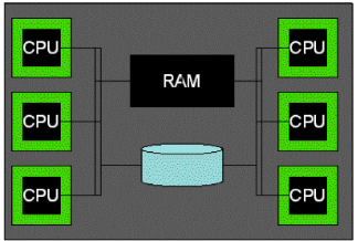
How are these machines connected together? The most straightforward option would probably be to have every CPU share memory and disk. This is called shared memory.

Another option is for each CPU to have its own memory, but all of them share the same disk. This is called shared disk.

.

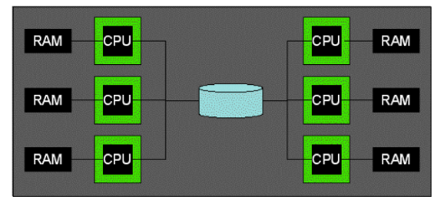These architectures are easy to reason about, but sharing resources holds back the system. It is possible to achieve a much higher level of parallelism if all the machines have their own disk and memory because they do not need to wait for the resource to become available. This architecture is called shared nothing and will be the architecture we use throughout the rest of the note.

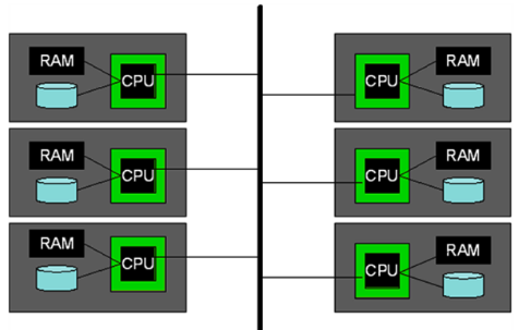
In shared nothing, the machines communicate with each other solely through the network by passing messages to each other.

Types of Parallelism

The focus of this note will be on intra-query parallelism. Intra-query parallelism attempts to make one query run as fast as possible by spreading the work over multiple computers. The other major type of parallelism is inter-query parallelism which gives each machine different queries to work on so that the system can achieve a high throughput and complete as many queries as possible. This may sound simple, but doing it correctly is actually quite difficult and we will address how to do it when we get to the module on concurrency.

Types of Intra-query Parallelism

We can further divide Intra-query parallelism into two classes: intra-operator and inter-operator. Intra-operator is making one operator run as quickly as possible. An example of intra-operator parallelism is dividing up the data onto several machines and having them sort the data in parallel. This parallelism makes sorting (one operation) as fast as possible. Inter-operator parallelism is making a query run as fast as possible by running the operators in parallel. For example, imagine our query plan looks like this:

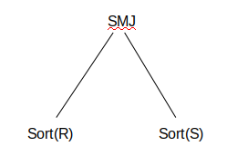
One machine can work on sorting R and another machine can sort S at the same time. In inter-operator parallelism, we parallelize the entire query, not individual operators.

Types of Inter-operator Parallelism

The last distinction we will make is between the different forms of inter-operator parallelism. The first type is pipeline parallelism. In pipeline parallelism records are passed to the parent operator as soon as they are done. The parent operator can work on a record that its child has already processed while the child operator is working on a different record. As an example, consider the query plan:

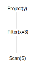
In pipeline parallelism the project and filter can run at the same time because as soon as filter finishes a record, project can operate on it while filter picks up a new record to operate on. The other type of inter-operator parallelism is bushy tree parallelism in which different branches of the tree are run in parallel. The example in section 3.1 where we sort the two files independently is an example of bushy tree parallelism. This is another example of bushy tree parallelism:

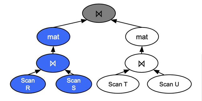
In bushy tree parallelism, the left branch and right branch can execute at the same time. For instance, scanning R, S, T, U can all happen at the same time. After that, joining R with S and joining T with U can happen in parallel as well.

Partitioning

Because all of our machines have their own disk we have to decide what data is stored on what machine. In this class each data page will be stored on only one machine. In industry we call this sharding and it is used to achieve better performance. If each data page appeared on multiple machines it would be called replication. This technique is used to achieve better availability (if one machine goes down another can handle requests), but it presents a host of other challenges that we will not study in depth in this class.

To decide what machines get what data we will use a partitioning scheme. A partitioning scheme is a rule that determines what machine a certain record will end up on. The three we will study are range partitioning, hash partitioning, and round-robin.

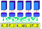
Range Partitioning

In a range partitioning scheme each machine gets a certain range of values that it will store (i.e. machine 1 will store values 1-5, machine 2 will store values 6-10, and so on).

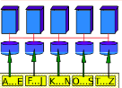
This scheme is very good for queries that lookup on a specific key (especially range queries compared to the other schemes we’ll talk about) because you only need to request data from the machines that the values reside on. It’s one of the schemes we use for parallel sorting and parallel sort merge join.

Hash Partitioning

In a hash partitioning scheme, each record is hashed and is sent to a machine matches that hash value. This means that all like values will be assigned to the same machine (i.e. if value 4 goes to machine 1 then all of the 4s must go to that machine), but it makes no guarantees about where close values go.

It will still perform well for key lookup, but not for range queries (because every machine will likely need to be queried). Hash partitioning is the other scheme of choice for parallel hashing and parallel hash join.

Round Robin Partitioning

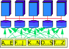
The last scheme we will talk about is called round robin partitioning. In this scheme we go record by record and assign each record to the next machine. For example the first record will be assigned to the first machine, the second record will be assigned to the second machine and so on. When we reach the final machine we will assign the next record to the first machine.

This may sound dumb but it has a nice property - every machine is guaranteed to get the same amount of data. This scheme will actually achieve maximum parallelization. The downside, of course, is that every machine will need to be activated for every query.

Network Cost

So far in this class we have only measured performance in terms of IOs. When we have multiple machines communicating over a network, however, we also need to consider the network cost. The network cost is how much data we need to send over the network to do an operation. Here network can be thought of as the space of communication among machines. It is different from memory and disk, which is why network cost is counted separately from I/O cost. Network cost is incurred whenever one machine sends data to another machine. In this class it is usually measured in KB. One important thing to note is that there is no requirement that entire pages must be sent over the network (unlike when going from memory to disk), so it is possible for the network cost to just be 1 record worth of data.

Partitioning Practice Questions

Assume that we have 5 machines and a 1000 page students(sid, name, gpa) table. Initially, all of the pages start on one machine. Assume pages are 1KB.

1) How much network cost does it take to round-robin partition the table?

2) How many IOs will it take to execute the following query:

    SELECT * FROM students where name = 'Josh Hug';

3) Suppose that instead of round robin partitioning the table, we hash partitioned it on the name column instead, How many IOs would the query from part 2 take?

4) Assume that an IO takes 1ms and the network cost is negligible. How long will the query in part 2 take if the data is round-robin partitioned and if the data is hash partitioned on the name column?

Now assume in the general case that we have \(n\) machines and \(p\) pages, all pages start on one machine, and that each pages is \(k\) KB. Express answers in terms of \(n\), \(p\), and \(k\).

5) How much network cost does it take to round-robin partition the table?

6) What is the minimum possible network cost to hash partition the table?

7) What is the maximum possible network cost to hash partition the table?

8) Now assume pages are randomly distributed across machines instead of all starting on one machine. Let the \(i\)th machine contain \(p_i\) pages such that \(\sum_{i=1}^{n} p_i = p\). How much network cost does it take to hash partition the table across all machines in the average case?

Partitioning Practice Solutions

1) In round robin partitioning the data is distributed completely evenly. This means that the machine the data starts on will be assigned 1/5 of the pages. This means that 4/5 of the the pages will need to move to different machines, so the answer is: 4/5 * 1000 * 1 = 800 KB.

2) When the data is round robin partitioned we have no idea what machine(s) the records we need will be on. This means we will have to do full scans on all of the machines so we will have to do a total of 1000 IOs.

3) When the data is hash partitioned on the name column, we know exactly what machine to go to for this query (we can calculate the hash value of ‘Josh Hug’ and find out what machine is assigned that hash value). This means we will only have to a full scan over 1 machine for a total of 200 IOs. Of course, this assumes all records with value ‘Josh Hug’ can fit on one machine.

4) Under both partitioning schemes it will take 200ms. Each machine will take the same amount of time to do a full scan, and all machines can be run at the same time so for runtime it doesn’t matter how many machines we need to query¹.

5) We send \(\frac{n-1}{n}\) of the pages to other machines, leaving \(\frac{1}{n}\) at the starting machine. Therefore, the network cost is then \(\frac{pk(n-1)}{n}\).

6) In the minimum possible network cost, all tuples hash to the starting machine so we do not need to send any tuples to other machines, resulting in a minimum network cost of 0.

7) In the minimum possible network cost, all tuples hash to other machines machine so we need to send all tuples to other machines, resulting in a maximum network cost of pk.

8) In the average case, each machine will hash \(\frac{n-1}{n}\) of its pages to other machines, resulting in a network cost of \(\frac{n-1}{n}\sum_{i=1}^{n} p_{i}k = \frac{pk(n-1)}{n}\).

Parallel Sorting

Let’s start speeding up some algorithms we already know by parallelizing them. There are two steps for parallel sorting:

1. Range partition the table

2. Perform local sort on each machine

We range partition the table because then once each machine sorts its data, the entire table is in sorted order (the data on each machine can be simply concatenated together if needed).

Generally, it will take (1 pass to partition the table across machines) + (number of passes needed to sort table) passes to parallel sort a table. This is equivalent to \(1 + \lceil1+\log_{B-1}\lceil N/mB\rceil\rceil\) passes (where m is the number of machines) to sort the data in the best case.

Parallel Hashing

Parallel hashing is very similar to parallel sorting. The two steps are:

1. Hash partition the table

2. Perform local hashing on each machine

Hash partitioning the table guarantees that like values will be assigned to the same machine. It would also be valid to range partition the data (because it has the same guarantee). However, in practice, range partitioning is a little harder (how do you come up with the ranges efficiently?) than hash-partitioning so use hash partitioning when possible.

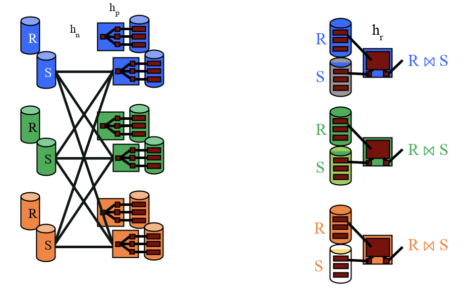
Parallel Sort Merge Join

The two steps for parallel sort merge join are:

1. Range partition each table using the same ranges on the join column

2. Perform local sort merge join on each machine

We need to use the same ranges to guarantee that all matches appear on the same machine. If we used different ranges for each table, then it’s possible that a record from table R will appear on a different machine than a record from table S even if they have the same value for the join column which will prevent these records from ever getting joined.

The total number of passes for parallel SMJ is (1 pass/table to partition across machines) + (number of passes needed to sort R) + (number of passes to sort S) + (1 final merge sort pass, going through both tables). This is \(2 + \lceil1+\log_{B-1}\lceil R/mB\rceil\rceil + \lceil1+\log_{B-1}\lceil S/mB\rceil\rceil + 2\) passes (where m is the number of machines).

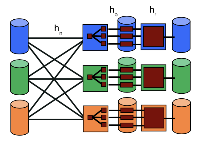
Parallel Grace Hash Join

The two steps for parallel hash join are:

1. Hash partition each table using the same hash function on the join column

2. Perform local grace hash join on each machine

Similarly to parallel SMJ, we need to use the same hash function for both tables to guarantee that matching records will be partitioned to the same machines.

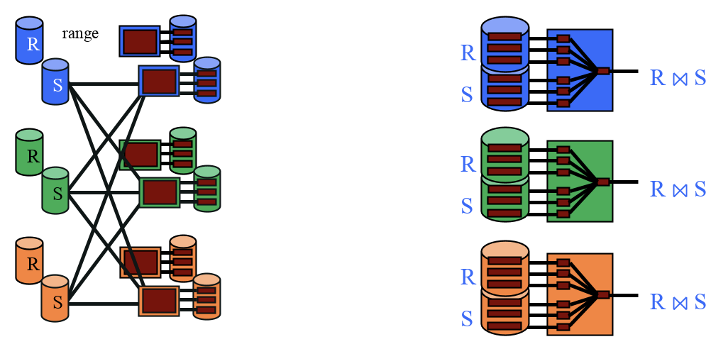
Broadcast Join

Let’s say we want to join a 1,000,000 page table that is currently round robin partitioned with a 100 page table that is currently all stored on one machine. We could do one of the parallel join algorithms discussed above, but to do this we would need to either range partition or hash partition the tables. It will take a ton of network cost to partition the big table.

Instead, we can use a broadcast join. A broadcast join will send the entire small relation to every machine, and then each machine will perform a local join. The concatenation of the results from each machine will be the final result of the join. While this algorithm has each machine operate on more data, we make up for this by sending much less data over the network. When we’re joining together one really large table and one small table, a broadcast join will normally be the fastest because of its network cost advantages.

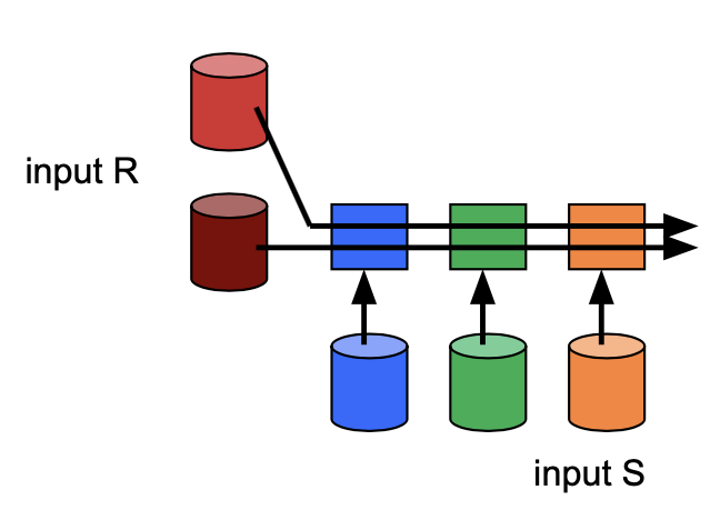
For instance, if relation R is small, we could do a broadcast join by sending R to all machines that have a partition of S. We perform a local join at each machine and union the results.

Symmetric Hash Join

The parallel joins we have discussed so far have been about making the join itself run as fast as possible by distributing the data across multiple machines. The problem with the join algorithms we have discussed so far is that they are pipeline breakers. This means that the join cannot produce output until it has processed every record. Why is this a problem? It prevents us from using pipeline parallelism. The operators above cannot work in parallel to the join because the join is taking a lot of time and then producing all of the output at once.

Sort Merge Join is a pipeline breaker because sorting is a pipeline breaker. You cannot produce the first row of output in sorting until you have seen all the input (how else would you know if your row is really the smallest?). Hash Join is a pipeline breaker because you cannot probe the hash table of each partition until you know that hash table has all the data in it. If you tried to probe one of the hash tables after processing only half the data, you might get only half of the matches that you should! Let’s try to build a hash based join that isn’t a pipeline breaker.

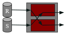
Symmetric Hash Join is a join algorithm that is pipeline-friendly, we can start producing output as soon as we see our first matches. Here are the steps to symmetric hash join:

1. Build two hash tables, one for each table in the join

2. When a record from R arrives, probe the hash table for S for all of the matches. When a record from S arrives, probe the hash table for R for all of the matches.

3. Whenever a record arrives add it to its corresponding hash table after probing the other hash table for matches.

This works because every output tuple gets generated exactly once - when the second record in the match arrives! But we produce output as soon as we see a match so it’s not a pipeline breaker.

Hierarchical Aggregation

The final parallel algorithm we’ll discuss is called hierarchical aggregation. Hierarchical aggregation is how we parallelize aggregation operations (i.e. SUM, COUNT, AVG). Each aggregation is implemented differently, so we’ll only discuss two in this section, but the ideas should carry over to the other operations easily.

To parallelize COUNT, each machine individually counts their records. The machines all send their counts to the coordinator machine who will then sum them together to figure out the overall count.\

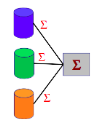
AVG is a little harder to calculate because the average of a bunch of averages isn’t necessarily the average of the data set. To parallelize AVG each machine must calculate the sum of all the values and the count. They then send these values to the coordinator machine. The coordinator machine adds up the sums to calculate the overall sum and then adds up the counts to calculate the overall count. It then divides the sum by the count to calculate the final average.

Parallel Algorithms Practice Questions

For 1 and 2, assume we have a 100 page table R that we will join with a 400 page table S. All the pages start on machine 1, and there are 4 machines in total with 30 buffer pages each.

1) How many passes are needed to do a parallel unoptimized SMJ on the data? For this question a pass is defined as a full pass over either table (so if we have to do 1 pass over R and 1 pass over S it is 2 total passes).

2) How many passes are needed to a parallel Grace Hash Join on the data?

3) We want to calculate the max in parallel using hierarchical aggregation. What value should each machine calculate and what should the coordinator do with those values?

4) If instead we had a 10000 page table R round-robin partitioned across 10 machines and the same 400 page table S on machine 1, what type of join would be appropriate for an equijoin?

5) If we used a non-uniform hash function which resulted in an uneven hash partition of our records, how will this affect the total time it takes to run parallel Grace Hash Join?

6) Consider a parallel version of Block Nested Loop Join in which we first range partition tuples from both tables and then perform BNLJ on each individual machine. Is this parallel algorithm pipeline friendly?

Parallel Algorithms Practice Solutions

1) 2 passes to partition the data (1 for each table). Each machine will then have 25 pages for R and 100 pages for S. R can be sorted in 1 pass but S requires 2 passes. Then it will take 2 passes to merge the tables together (1 for each table). This gives us a total of 2 (partition) + 1 (sort R) + 2 (sort S) + 2 (merge relations) = 7 passes.

2) Again we will need 2 passes to partition the data across the four machines and each machine will have 25 pages for R and 100 for S. We don’t need any partitioning passes because R fits in memory on every machine, so we only need to do build and probe, which will take 2 passes (1 for each table). This gives us a total of 4 passes.

3) Each machine should calculate the max and the coordinator will take the max of those maxes.

4) A broadcast join since this type of join helps reduce network costs when we have two tables with drastically different sizes and the larger one is split into many machines.

5) The parallel join algorithm would only finish when the last machine finishes its Grace Hash Join. This last machine is likely to be the machine that received the most pages from the partitioning phase since it may take more I/Os to hash it.

6) No, because if BNLJ runs for each block of the outer relation R, we need scan through the inner relation S to find matching tuples and thus, we would need the machine to have all of S first before we can begin the join. Therefore, this is a pipeline breaker.

Past Exam Problems

• Fa22 Final Question 9

• Sp22 Final Question 9

• Fa21 Final Question 10

• Sp21 Final Question 4b, 8bi

• Fa20 Final Question 6

1. In reality, there may be some variance in how long each machine takes to complete a scan, and the likelihood of a "straggler" (i.e. slow machine) increases with the number of machines involved in a query, but for simplicity we ignore this detail ↩