Introduction

When we covered SQL, we gave you a helpful mental model for how queries are executed. First you get all the rows in the FROM clause, then you filter out columns you don’t need in the WHERE clause, and so on. This was useful because it guarantees that you will get the correct result for the query, but it is not what databases actually do. Databases can change the order they execute the operations in order to get the best performance. Remember that in this class, we measure performance in terms of the number of I/Os. Query Optimization is all about finding the query plan that minimizes the number of I/Os it takes to execute the query. A query plan is just a sequence of operations that will get us the correct result for a query. We use relational algebra to express it. This is an example of a query plan:

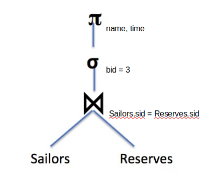
First it joins the two tables together, then it filters out the rows, and finally it projects only the columns it wants. As we’ll soon see, we can come up with a much better query plan!

Iterator Interface

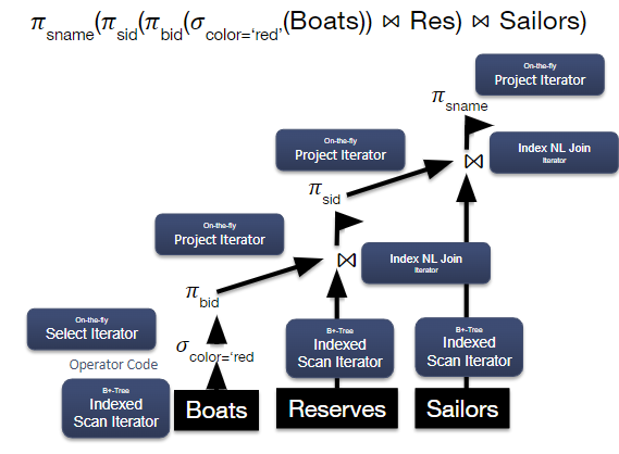
The expression tree above is representative of some query plan, where the edges encode the “flow” of tuples, the vertices represent relational algebra operators, and the source vertex represents a table access operator. For some SQL query, there may be multiple ways to receive the same output; the goal of a query optimizer is to generate a sequence of operators that returns the correct output efficiently. Once this sequence is generated, the query executor then creates instances of each operator, each of which implements an iterator interface. The iterator interface is responsible for efficiently executing operator logic and forwarding relevant tuples to next operator.
Every relational operator is implemented as a subclass of the Iterator class, so in executing a query plan, we will call next() on the root operator, and recurse down until the base case. For example, in the diagram below, the root operator (SELECT sname) will call next(), which will recursively call next() for the join iterator, which recursively calls next() down the query until we reach the base case. We call this a pull-based computation model. Each time we call next(), we will either perform a streaming ("on-the-fly") or blocking ("batch") algorithm on the operator instance. Streaming operators use a small amount of work to produce each tuple, like a SELECT statement. Blocking operators like sort operations, on the other hand, do not produce output until they consume their entire input.

In this way, we can see how query plans are single-threaded: we simply recursively call next() on the query plan until we reach our base operator.

Selectivity Estimation

An important property of query optimization is that we have no way of knowing how many I/Os a plan will cost until we execute that plan. This has two important implications. The first is that it is impossible for us to guarantee that we will find the optimal query plan - we can only hope to find a good (enough) one using heuristics and estimations. The second is that we need some way to estimate how much a query plan costs. One tool that we will use to estimate a query plan’s cost is called selectivity estimation. The selectivity of an operator is an approximation for what percentage of pages will make it through the operator onto the operator above it. This is important because if we have an operator that greatly reduces the number of pages that advance to the next stage (like the WHERE clause), we probably want to do that as soon as possible so that the other operators have to work on fewer pages.

Most of the formulas for selectivity estimation are fairly straightforward. For example, to estimate the selectivity of a condition of the form \(X=3\), the formula is 1 / (number of unique values of X). The formulas used in this note are listed below, but please see the lecture/discussion slides for a complete list. The last section of this note also contains the important formulas. In these examples, capital letters are for columns and lowercase letters represent constants. All values in the following examples are integers, as floats have different formulas.

X=a: 1/(unique vals in X)
X=Y: 1/max(unique vals in X, unique vals in Y)
X\(>\)a: (max(X) - a) / (max(X) - min(X) + 1)
cond1 AND cond2: Selectivity(cond1) * Selectivity(cond2)

Selectivity of Joins

Let’s say we are trying to join together tables A and B on the condition A.id = B.id. If there was no condition, there would be \(|A| * |B|\) tuples in the result, because without the condition, every row from A is joined with every row from B and all the rows will be included in the output. However, taking the join condition into account, some of the rows will be not be included into the output. In order to estimate the number of rows that will be included in the output after the join condition X=Y, we use the selectivity estimation: 1/max(unique vals for A.id, unique vals for B.id), meaning that the total number of tuples we can expect to move on is:

\[\frac{|A| * |B|}{max(unique \ vals \ for \ A.id, \ unique \ vals \ for \ B.id)}\]

To find a join’s output size in pages, we need to follow 3 steps:

Find the join’s selectivity. For a join on tables A and B on the condition A.id = B.id, we can refer to the formula above for this.
Find the estimated number of joined tuples in the output by multiplying the selectivity of the join by the number of joined tuples in the Cartesian Product between the two tables.
Find the estimated number of pages in the join output by dividing by the estimated number of joined tuples per page.

Note that we cannot directly multiply the selectivity by the number of pages in each table that we are joining to find the estimated output size in pages. To see why, suppose we had two relations, \(R\) and \(S\), with only 1 page each and 5 tuples per page \(\left([R] = [S] = 1,\ |R| = |S| = 5 \right)\). For simplicity, let’s also assume that the join’s selectivity is \(1\) (i.e. all the tuples in the Cartesian Product between \(R\) and \(S\) are in the output). Then, the number of output tuples would equal the number of tuples in the Cartesian Product: \(|R| * |S| = 5 * 5 = 25\). In this example, \(25\) joined tuples would take up more space than the \([R] * [S] = 1\) page estimate we would get if we directly multiplied the number of pages in each relation!

Common Heuristics

There are way too many possible query plans for a reasonably complex query to analyze them all. We need some way to cut down the number of plans that we actually consider. For this reason, we will use a few heuristics:

Push down projects (\(\pi\)) and selects (\(\sigma\)) as far as they can go
Only consider left deep plans
Do not consider cross joins unless they are the only option

The first heuristic says that we will push down projects and selects as far as they can go. We touched on why pushing down selects will be beneficial. It reduces the number of pages the other operators have to deal with. But why is pushing projects down beneficial? It turns out this also reduces the number of pages future operators need to deal with. Because projects eliminate columns, the rows become smaller, meaning we can fit more of them on a page, and thus there are fewer pages! Note that you can only project away columns that are not used in the rest of the query (i.e. if they are in a SELECT or a WHERE clause that hasn’t yet been evaluated you can’t get rid of the column).

The second heuristic says to only consider left deep plans. A left deep plan is a plan where all of the right tables in a join are the base tables (in other words, the right side is never the result of a join itself, it can only be one of the original tables). The following diagram gives some examples of what are and what are not left-deep plans.

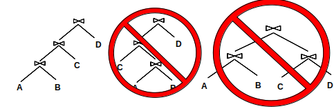
Left deep plans are beneficial for two main reasons. First, only considering them greatly reduces the plan space. The plan space is factorial in the number of relations, but it is a lot smaller than it would be if we considered every plan. Second, these plans can be fully pipelined, meaning that we can pass the pages up one at a time to the next join operator – we don’t actually have to write the result of a join to disk.

The third heuristic is beneficial because cross joins produce a ton of pages which makes the operators above the cross join perform many I/Os. We want to avoid that whenever possible.

Pass 1 of System R

The query optimizer that we will study in this class is called System R. System R uses all of the heuristics that we mentioned in the previous section. The first pass of System R determines how to access tables optimally or interestingly (we will define interesting in a bit).

We have two options for how to access tables during the first pass:

Full Scan
Index Scan (for every index the table has built on it)

For both of these scans, we only return a row if it matches all of the single table conditions pertaining to its table because of the first heuristic (push down selects). A condition involving columns from multiple tables is a join condition and cannot yet be applied because we’re only considering how to access individual tables. This means the selectivity for each type of scan is the same, because they are applying the same conditions!

The number of I/Os required for each type of scan will not be the same, however. For a table P, a full scan will always take [P] I/Os; it needs to read in every page.

For an index scan, the number of I/Os depends on how the records are stored and whether or not the index is clustered. Alternative 1 indexes have an IO cost of:

(cost to reach level above leaf) + (num leaves read)

You don’t necessarily have to read every leaf, because you can apply the conditions that involve the column the index is built on. This is because the data is in sorted order in the leaves, so you can go straight to the leaf you should start at, and you can scan right until the condition is no longer true.

Example: Important information:

Table A has [A] pages
There is an alternative 1 index built on C1 of height 2
There are 2 conditions in our query: C1 \(>\) 5 and C2 \(<\) 6
C1 and C2 both have values in the range 1-10

The selectivity will be 0.25 because both conditions have selectivity 0.5 (from selectivity formulas), and it’s an AND clause so we multiply them together. However, we can not use the C2 condition to narrow down what pages we look at in our index because the index is not built on C2. We can use the C1 condition, so we only have to look at 0.5[A] leaf pages. We also have to read the two index pages to find what leaf to start at, for a total number of 2 + 0.5[A] I/Os.

For alternative 2/3 indexes, the formula is a little different. The new formula is:

(cost to reach level above leaf) + (num of leaf nodes read) + (num of data pages read).

We can apply the selectivity (for conditions on the column that the index is built on) to both the number of leaf nodes read and the number of data pages read. For a clustered index, the number of data pages read is the selectivity multiplied by the total number of data pages. For an unclustered index, however, you have to do an IO for each record, so it is the selectivity multiplied by the total number of records.

Example: Important information:

Table B with B data pages and \(\\|B\\|\) records
Alt 2 index on column C1, with a height of 2 and [L] leaf pages
There are two conditions: C1 \(>\) 5 and C2 \(<\) 6
C1 and C2 both have values in the range 1-10

If the index is clustered, the scan will take 2 I/Os to reach the index node above the leaf level, it will then have to read 0.5[L] leaf pages, and then 0.5[B] data pages. Therefore, the total is 2 + 0.5[L] + 0.5[B]. If the index is unclustered, the formula is the same except we have to read 0.5\(|B|\) data pages instead. So the total number of I/Os is 2 + 0.5[L] + 0.5\(|B|\).

The final step of pass 1 is to decide which access plans we will advance to the subsequent passes to be considered. For each table, we will advance the optimal access plan (the one that requires the fewest number of I/Os) and any access plans that produce an optimal interesting order. An interesting order is when the table is sorted on a column that is either:

Used in an ORDER BY
Used in a GROUP BY
Used in a downstream join (a join that hasn’t yet been evaluated. For pass 1, this is all joins).

The first two are hopefully obvious. The last one is valuable because it can allow us to reduce the number of I/Os required for a sort merge join later on in the query’s execution. A full scan will never produce an interesting order because its output is not sorted. An index scan, however, will produce the output in sorted order on the column that the index is built on. Remember though, that this order is only interesting if it used later in our query!

Example: Let’s say we are evaluating the following query:

SELECT * 
FROM players INNER JOIN teams
ON players.teamid = teams.id
ORDER BY fname;

And we have the following potential access patterns:

Full Scan players (100 I/Os)
Index Scan players.age (90 I/Os)
Index Scan players.teamid (120 I/Os)
Full Scan teams (300 I/Os)
Index Scan teams.record (400 I/Os)

Patterns 2, 3, and 4 will move on. Patterns 2 and 4 are the optimal pattern for their respective table, and pattern 3 has an interesting order because teamid is used in a downstream join.

Passes 2..n

The rest of the passes of the System R algorithm are concerned with joining the tables together. For each pass i, we attempt to join i tables together, using the results from pass i-1 and pass 1. For example, on pass 2 we will attempt to join two tables together, each from pass 1. On pass 5, we will attempt to join a total of 5 tables together. We will get 4 of those tables from pass 4 (which figured out how to join 4 tables together), and we will get the remaining table from pass 1. Notice that this enforces our left-deep plan heuristic. We are always joining a set of joined tables with one base table.

Pass i will produce at least one query plan for all sets of tables of length i that can be joined without a cross join (assuming there is at least one such set). Just like in pass 1, it will advance the optimal plan for each set, and also the optimal plan for each interesting order for each set (if one exists). When attempting to join a set of tables with one table from pass 1, we consider each join the database has implemented.

Only one of these joins produces a sorted output - sort merge join (SMJ), so the only way to have an interesting order is by using SMJ for the last join in the set. The output of SMJ will be sorted on the columns in the join condition.

However, both simple nested loop join (SNLJ) and index nested loop join (INLJ) can preserve a sorted ordering of the left relation. Since both of these perform all the joins on an individual tuple from the left relation before moving to the next tuple from left relation, the left relation’s ordering is preserved.

Grace Hash Join (GHJ), Page Nested Loop Join (PNLJ), and Block Nested Loop Join (BNLJ) never produce an interesting ordering. GHJ’s output order is based on the order of tuples in the probing relation since we iterate through each tuple in the probing relation to find matches in the other relation’s in-memory hash table. However, since the probing relation itself has been partitioned by hashing, there are no guarantees about the probing relation’s ordering across partitions, so there are no guarantees about the output’s overall ordering. PNLJ and BNLJ are similar to SNLJ, but they don’t generate all the join outputs of a single tuple in the left relation before moving to the next tuple in the left relation. Instead, they read ranges of tuples from the left relation and make matches on these ranges with chunks of tuples from the right relation, so they don’t preserve order.

Example: We are trying to execute the following query:

SELECT * 
FROM A INNER JOIN B
ON A.aid = B.bid 
INNER JOIN C
ON b.did = c.cid
ORDER BY c.cid;

Which sets of tables will we return query plans for in pass 2? The only sets of tables we will consider on this pass are {A, B} and {B, C}. We do not consider {A, C} because there is no join condition and our heuristics tell us not to consider cross joins. To simplify the problem, let’s say we only implemented SMJ and BNLJ in our database and that pass 1 only returned a full table scan for each table. These are the following joins we will consider (the costs are made up for the problem. In practice you will use selectivity estimation and the join cost formulas):

A BNLJ B (estimated cost: 1000)
B BNLJ A (estimated cost: 1500)
A SMJ B (estimated cost: 2000)
B BNLJ C (estimated cost: 800)
C BNLJ B (estimated cost: 600)
C SMJ B (estimated cost: 1000)

Joins 1, 5, and 6 will advance. 1 is the optimal join for the set {A, B}. 5 is optimal for the set {B, C}. 6 is an interesting order because have an ORDER BY clauses that uses c.cid later in the query. We don’t advance 3 because A.aid and B.bid are not used after that join so the order isn’t interesting.

Now let’s go to pass 3. We will consider the following joins (again join costs are made up):

Join 1 {A, B} BNLJ C (estimated cost: 10,000)
Join 1 {A, B} SMJ C (estimated cost: 12,000)
Join 5 {B, C} BNLJ A (estimated cost 8,000)
Join 5 {B, C} SMJ A (estimated cost: 20,000)
Join 6 {B, C} BNLJ A (estimated cost: 22,000)
Join 6 {B, C} SMJ A (estimated cost: 18,000)

Notice that now we can’t change the join order, because we are only considering left deep plans, so the base tables must be on the right.

The only plans that will advance now are 2 and 3. 3 is optimal overall for the set of all 3 tables. 2 is optimal for the set of all 3 tables with an interesting order on C.cid (which is still interesting because we haven’t evaluated the ORDER BY clause). The reason 2 produces the output sorted on C.cid is that the join condition is B.did = C.cid, so the output will be sorted on both B.did and C.cid (because they are the same). 4 and 6 will not produce output sorted on C.cid because they will be adding A to the set of joined tables so the condition will be A.aid = B.bid. Neither A.aid nor B.bid are used elsewhere in the query, so their ordering is not interesting to us.

Calculating I/O Costs for Join Operations

When we are estimating the I/O costs of the queries we are trying to optimize, it is important to consider the following:

Whether we materialize intermediate relations (outputs from previous operators) or stream them into the input of the next operator.
If interesting orders obtained from previous operators may reduce the I/O cost of performing a join.

Due to these considerations, we may not be able to directly use the formulas from the Iterators & Joins module to calculate I/O cost.

Consideration #1

Whether we materialize intermediate relations (outputs from previous operators) or stream them into the input of the next operator can affect the I/O cost of our query.

To materialize intermediate relations, we write the output of an intermediate operator to disk (i.e. writing it to a temporary file), a process that incurs additional I/Os. When this data is passed onto the next operator, we must read it from disk into memory again. On the other hand, if we stream the output of one operator into the next, we do not write the intermediate outputs to disk. Instead, as soon as tuples become available when we process the first operator, they remain in memory and we begin applying the second operator to them.

For example, when we push down selections/projections, our goal is to reduce the size of our data so that fewer I/Os are necessary for reading in this data as we traverse up the tree. However, we will only see an impact in I/O cost if the outputs of these selections/projections are materialized, or if the next operator we perform only makes a single pass through the data (i.e. left relations of S/P/BNLJ, left relation of INLJ, etc.). To illustrate this, let’s look at the following example.

Example:
Assume B = 5, [P] = 50, [T] = 100, there are 30 pages of players records where P.teamid \(>\) 200, and there are 40 pages worth of records where T.tname \(>\) ‘Team5’. We are optimizing the following query:

SELECT * 
FROM players P INNER JOIN teams T
ON P.teamid = T.teamid
WHERE P.teamid > 200 AND T.tname > `Team5';

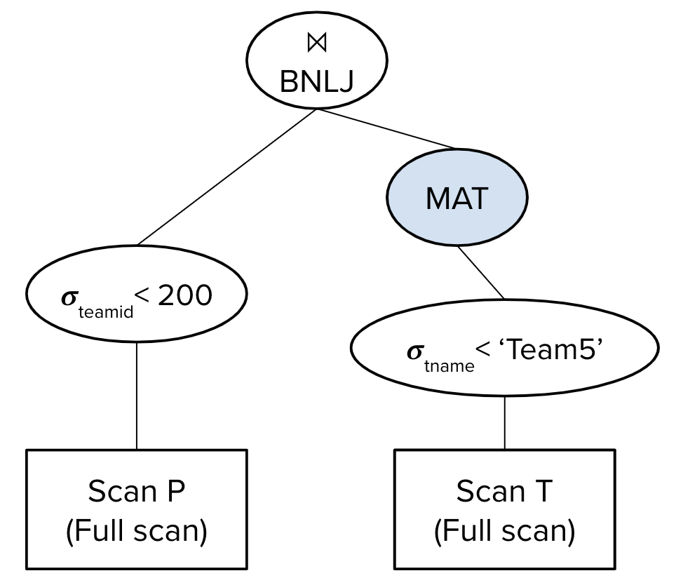
Suppose our query optimizer chose the following query plan:

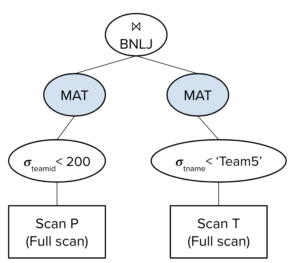
The estimated I/O cost of this query plan would be \((50 + 30) + (100 + 40) + (30 + \left\lceil \frac{30}{5-2}\right\rceil * 40) = 650\) I/Os.

We first perform a full scan on P: we read in all 50 pages of P, identify the records where P.teamid \(>\) 200, and write the 30 pages of those records to disk. This happens because we are materializing the output we get after the selection. We repeat the same process for T: we read in all 100 pages of T, identify the records where T.tname \(>\) ‘Team5’, and write the 40 pages of those records to disk.

Next, when we join the two tables together with BNLJ, we are working with the 30 pages of P and 40 pages of T that the selections have been applied to and currently lie on disk. For each block of B-2 pages of P, we read in all of T, hence the \((30 + \left\lceil \frac{30}{5-2}\right\rceil * 40)\) term.

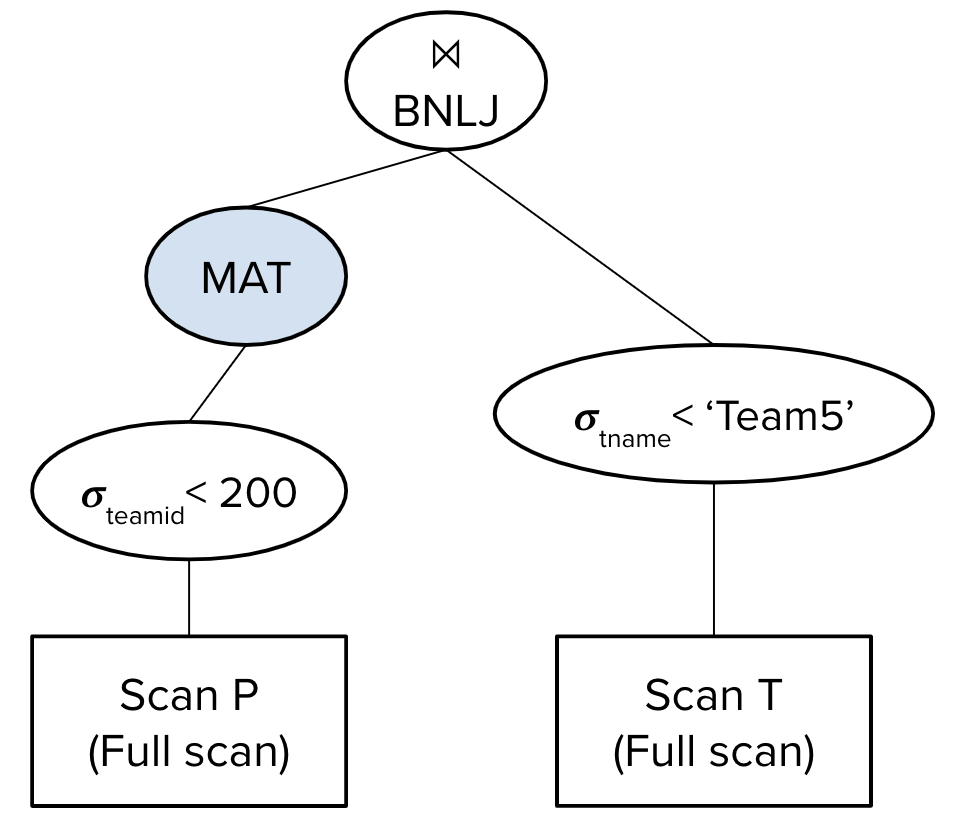
Now, suppose our query optimizer instead chose the following query plan:

The estimated I/O cost of this query plan would be \((100 + 40) + (50 + \left\lceil \frac{30}{5-2}\right\rceil * 40) = 590\) I/Os.

Since we materialize the output we get after performing the selection on T, we first read in all 100 pages of T, identify the records where T.tname \(>\) ‘Team5’, and write the 40 pages of those records to disk.
Then, we perform a full scan over P, reading in each of the 50 pages into memory. This costs 50 I/Os, and we will filter for records with P.teamid \(<\) 200 in memory. Once we’ve identified a block of B-2 pages of P where P.teamid \(<\) 200, we need to find the matching records in T by reading in the 40 pages of T from disk that were materialized after the selection on T.tname \(<\) ‘Team5’. This process repeats for every block of P, and since we have 30 pages of records where P.teamid \(<\) 200 and each block has size B-2, there are approximately \(\left\lceil \frac{30}{5-2}\right\rceil\) blocks of P to process.

This is why the cost of the BNLJ is \(50 + \left\lceil \frac{30}{5-2}\right\rceil * 40\). This diverges from the BNLJ formula presented in the Iterators & Joins module: we read in all 50 pages of P, but because we push down the selection on P, only 30 pages of P will be passed along to the BNLJ operator and we only need to find matching T records for these pages.

Now, suppose our query optimizer instead chose the following query plan:

The estimated I/O cost of this query plan would be \((50 + 30) + (30 + \left\lceil \frac{30}{5-2}\right\rceil * 100) = 1110\) I/Os.

Since we materialize the output we get after performing the selection on P, we first read in all 50 pages of P, identify the records where P.teamid \(>\) 200, and write the 30 pages of those records to disk.

We will read in the 30 pages of P remaining after the selection in blocks of size B-2. For every block of P, we need to identify the matching records in T. Since we do not materialize after selecting records where tname \(<\) ‘Team5’, we will have to perform a full scan on the entire T table for every single block of P, reading in T page-by-page into memory, finding records where tname \(<\) ‘Team5’, and joining them with records in P. There are \(\left\lceil \frac{30}{5-2}\right\rceil\) blocks of P to process, hence the \(\left\lceil \frac{30}{5-2}\right\rceil * 100\) term.

Here, we see that even though we pushed down the selection on T, it did not impact the I/O cost of the query. The I/O cost would be the same if we used this query plan instead:

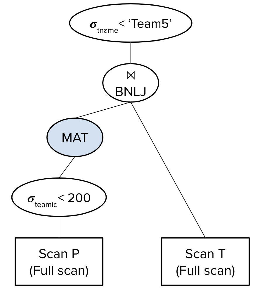
The reason why the I/O cost remains unaffected is that every time we make a pass through T (once per block of P), we still need to access the entire T table and apply the selection on the fly since we did not save these intermediate results. This shows how pushing down selections/projections affects our I/O cost only when the next operator makes a single pass through the data or when outputs of intermediate relations are materialized.

For the System R query optimizer we are studying in this class, assume that we never materialize the outputs of any intermediate operators and that they are streamed in as the input to the next operator.

Thus, this is the query plan that the System R query optimizer would consider:

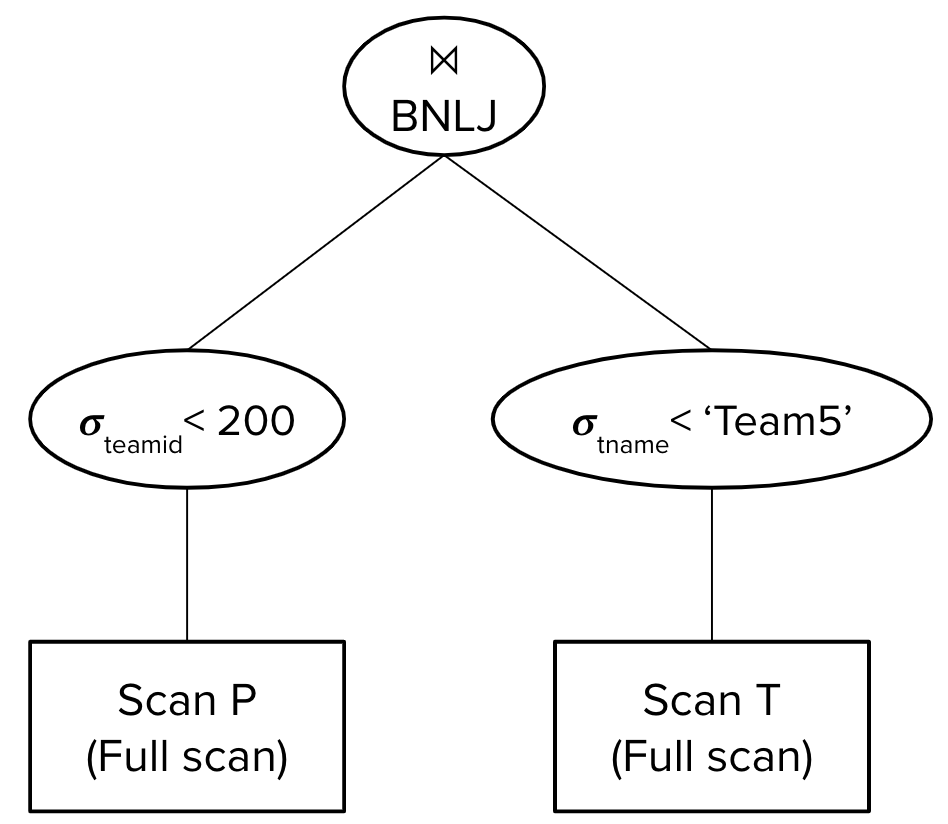
The estimated I/O cost of this query plan would be \(50 + \left\lceil \frac{30}{5-2}\right\rceil * 100 = 1050\) I/Os.

We perform a full scan over P, reading in each of the 50 pages into memory and filtering for records with P.teamid \(<\) 200. Since we push down this selection, only 30 pages of P will be passed onto the BNLJ operator. For every block of B-2 pages of P where P.teamid \(<\) 200, we need to identify the matching records in T. Since we do not materialize after selecting records where tname \(<\) ‘Team5’, we will have to perform a full scan on the entire T table for every single block of P, reading in T page-by-page into memory, finding records where tname \(<\) ‘Team5’, and joining them with records in P. There are \(\left\lceil \frac{30}{5-2}\right\rceil\) blocks of P to process, hence the \(\left\lceil \frac{30}{5-2}\right\rceil * 100\) term.

Consideration #2

We must also consider the effects of interesting orders from previous operators. For example, let’s say we are optimizing the following query, where the players table contains 50 pages and the teams table contains 100 pages:

SELECT * 
FROM players P INNER JOIN teams T
ON P.teamid = T.teamid
WHERE P.teamid > 200;

Suppose we push down the selection P.teamid \(>\) 200, choose an index scan on P.teamid costing 60 I/Os as our access plan for the P table, and choose a full scan costing 100 I/Os as our access plan for the T table. The output of the index scan will be sorted on teamid, which is an interesting order since it may be used in the downstream join between P and T.

Now, suppose that we choose SMJ as our join algorithm for joining together P and T. The formula that we presented in the Iterators & Joins module would estimate the I/O cost to be: cost to sort P + cost to sort T + (50 + 100), where the last term ([P] + [T]) is the average case cost of the merging step and accounts for the cost of reading in both tables.

However, if we use the index scan on P.teamid, we no longer need to run external sorting on P! Instead, we will account for the I/O cost of accessing P using the index scan and stream in the output of this index scan into the merging phase. Thus, the estimated cost of this query plan would be (cost to sort T + 60 + 100) I/Os.

Practice Questions

Given the following tables:

Teams (teamid, tname, currentcoach)
Players (playerid, pname, teamid, points)
Coaches (coachid, cname)

Answer questions 1-5 about the following query:

SELECT pname, cname
FROM Teams t
INNER JOIN Players p ON t.teamid = p.teamid
INNER JOIN Coaches c ON t.currentcoach = c.coachid
WHERE p.rating > 5
ORDER BY p.playerid;

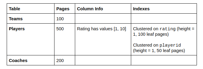
1) What is the selectivity of the p.rating \(>\) 5 condition?

2) What single table access plans will advance to the next pass?

Full scan on Teams
Full scan on Players
Index scan on Players.rating
Index scan on Players.playerid
Full scan on Coaches

3) Which of the following 2 table plans will advance from the second pass to the third pass? Assume that the I/Os provided is optimal for those tables joined in that order and also assume that the output of every plan is not sorted.

Teams Join Players (1000 I/Os)
Players Join Teams (1500 I/Os)
Players Join Coaches (2000 I/Os)
Coaches Join Players (800 I/Os)
Teams Join Coaches (500 I/Os)
Coaches Join Teams (750 I/Os)

4) Which of the following 3 table plans will be considered during the third pass? Again assume that the I/Os provided is optimal for joining the tables in that order and that none of the outputs are sorted.

(Teams Join Players) Join Coaches - 10,000 I/Os
Coaches Join (Teams Join Players) - 8,000 I/Os
(Players Join Teams) Join Coaches - 9,000 I/Os
(Players Join Coaches) Join Teams - 12,000 I/Os
(Teams Join Coaches) Join Players - 15,000, I/Os

5) Which 3 table plan will be used?

6) Now, suppose we are trying to optimize the following query using the System R query optimizer:

SELECT * 
FROM players P INNER JOIN teams T
ON P.teamid = T.teamid
WHERE P.teamid > 200 AND T.tname > `Team5';

Assume B = 5, [P] = 50, [T] = 100, there are 30 pages of players records where P.teamid \(>\) 200, and there are 40 pages worth of records where T.tname \(>\) ‘Team5’.
Also, assume that the access plans we chose in Pass 1 are:

Index scan on P.teamid: 60 I/Os
Full scan on T: 100 I/Os

Given this information, estimate the average case I/O cost of P SMJ T for Pass 2, assuming we are using unoptimized SMJ.

7) Suppose we run a custom optimizer on the following query:

SELECT * 
FROM students S INNER JOIN teachers T
ON s.schoolid = t.schoolid
WHERE s.absences > 10 AND t.days_worked < 50;

Assume B = 5, [S] = 20, and [T] = 30. Also assume that there are 12 pages of student records where s.absences \(>\) 10 and 15 pages of teachers records where t.days_worked \(<\) 50. Suppose that the System R optimizer decides to use a Block Nested Loop Join with an estimated 130 I/Os. Design a better query plan and calculate how many I/Os it saves compared to the System R plan.

Solutions

1) 1/2. You can use the formula in lecture/discussion slides, but these are often quicker to solve off the top of your head. Rating can be between 1 and 10 (10 values) and there are 5 values that are greater than 5 (6, 7, 8, 9, 10), so the selectivity is 5/10 or 1/2.

2) a, c, d, e. Every table needs at least one access plan to advance, and for Teams and Coaches there is only one option - the full scan. For Players the optimal plan will advance as well as the optimal plan with an interesting order on playerid (playerid is interesting to us because it is used in an ORDER BY later in the query). A full scan takes 500 I/Os. The scan on rating takes 1 + 0.5(100) + 0.5(500) = 301 I/Os. The scan on playerid takes 1 + 50 + 500 = 551 I/Os. The optimal access plan is the index scan on rating, so it advances, and the index scan on playerid is the only plan that produces output sorted on playerid so it advances as well.

3) a, e. First recognize that no plan that involves joining Players with Coaches will be considered because there is no join condition between them so it would be a cross join and we don’t consider cross joins unless they are our only option for that pass. Then we just pick the best plan for each set of tables which in this case is Teams Join Players for the (teams, players) set and Teams Join Coaches for the (Teams, Coaches) set.

4) a, e. B is not considered because it is not a left deep join. C and D both attempt to join 2 table plans that did not advance from pass 2 with a single table plan. A and E (the only correct answers) correctly join a 2 table plan from pass 2 with a single table plan and they are both left deep plans.

5) (Teams Join Players) Join Coaches. It has the fewest I/Os out of the plans we are considering. There is no potential for interesting orders because none of the results are sorted, so only one plan can advance.

6) ((100 + 40) + (40+40) + (40+40)) + 60 + 40 = 400 I/Os.
The cost of sorting T by T.teamid (to completion, since we are performing unoptimized SMJ) is (100 + 40) + (40+40) + (40+40) I/Os:

In Pass 0 of external sorting, we read in 100 pages of T, but apply the selection on T to the tuples in memory and only write sorted runs for the 40 pages of T that satisfy T.tname \(>\) ‘Team5’. With B=5, we will produce 8 sorted runs of 5 pages each. This costs 100 + 40 I/Os.
In Pass 1 of external sorting, we are able to merge B-1 = 4 sorted runs together at a time, producing 2 sorted runs. This costs 40 + 40 I/Os.
In Pass 2 of external sorting, we merge together the 2 sorted runs, producing 1 sorted run containing all our data. This costs 40 + 40 I/Os.

The access plan our query optimizer chose for P in Pass 1 is the index scan on P.teamid. This will produce output that is already sorted on P.teamid, so we don’t need to run external sorting on P. When we proceed to the merging phase of SMJ, we will account for the I/O cost of accessing P using this index scan (60 I/Os) and stream in its output to the merging phase. For T, we will read in the 40 pages from the final sorted run on disk produced after external sorting. Thus, the merging phase costs 60 + 40 I/Os in the average case.

Note: If we chose to apply the SMJ optimization, we would be able to achieve an I/O cost of ((100 + 40) + (40+40)) + 60 + 40 = 320 I/Os. Rather than sorting T to completion, we could stop after Pass 1 of external sorting so that we have 2 sorted runs of T that have not yet been merged together. Then, in the merging phase of SMJ, we allocate our 5 buffer pages the following way:

1 buffer page is reserved as the output buffer
Since we are performing the optimization, 2 buffer pages are reserved for reading in the runs of T. The data in the first run is read page-by-page into one buffer page, and the data in the second run is read page-by-page into the other buffer page.
We have 2 buffer pages left - these are used for the index scan on P. We can perform the index given only 2 buffer pages because if the index is Alternative 1, we will only need 1 buffer page to store the inner/leaf node currently being processed (it can be evicted as soon as we need to read in another node). If the index is Alternative 2 or 3, we will need 2 buffer pages because when scanning through leaf nodes and reading in the records on data pages, we need 1 page to store the data page and 1 page to store the leaf node. We need more than 1 buffer page because if we evict a leaf node and replace it with the data page a record lies on, we will not be able to efficiently find the next records without the leaf node in memory.

This problem doesn’t specify what alternative the index we’re using for the index scan is, but either way, 2 buffer pages will be sufficient for performing this index scan.

7) We can start by using a Block Nested Loop Join (BNLJ) with the teachers relation as the outer relation and the students relation as inner relation. We can then push down the selects on the predicates s.absences \(>\) 10 and t.days_worked \(<\) 50. To get better performance, we can also materialize the output of the select on the students relation, so we don’t have to keep reading the full relation on each loop. This gives us \(30 + 20 + 12 + \left\lceil \frac{15}{5 - 2} \right\rceil * 12 = 122\). This plan costs \(8\) I/Os less than the System R plan. Remember that System R doesn’t consider materializing intermediate outputs, so that’s one potential avenue to explore when trying to improve System R’s query plans.

Appendix - Selectivity Values

\(\\|c\\|\) is the number of distinct values in the column

Equalities

Predicate	Selectivity	Assumption
\(c=v\)	1 / (# of distinct values of \(c\) in index)	We know \(\|c\|\).
\(c=v\)	1/10	We don’t know \(\|c\|\).
\(c_1 = c_2\)	1 / max(# of distinct values of \(c_1\),# of distinct values of \(c_2\))	We know \(\|c_1\|\) and \(\|c_2\|\).
\(c_1 = c_2\)	1 / (# of distinct values of \(c_i\))	We know \(\|c_i\|\) but not \(\|\)other column\(\|\).
\(c_1 = c_2\)	1/10	We don’t know \(\|c_1\|\) or \(\|c_2\|\).

Inequalities on Integers

Predicate	Selectivity	Assumption
\(c<v\)	(v - min(\(c\))) / (max(\(c\)) - min(\(c\)) + 1)	We know max(\(c\)) and min(\(c\)).
\(c>v\)	(max(\(c\)) - v) / (max(\(c\)) - min(\(c\)) + 1)	\(c\) is an integer.
\(c<v\), \(c>v\)	1/10	We don’t know max(\(c\)) and min(\(c\)). \(c\) is an integer.
\(c <= v\)	(v - min(\(c\))) / (max(\(c\)) - min(\(c\)) + 1) + (1/\(\|c\|\))	We know max(\(c\)) and min(\(c\)).
\(c >= v\)	(max(\(c\)) - v) / (max(\(c\)) - min(\(c\)) + 1) + (1/\(\|c\|\))	\(c\) is an integer.
\(c <= v\), \(c >= v\)	1/10	We don’t know max(\(c\)) and min(\(c\)).\(c\) is an integer.

Inequalities on Floats

Predicate	Selectivity	Assumption
\(c>=v\)	(max(\(c\)) - v) / (max(\(c\)) - min(\(c\)))	We know max(\(c\)) and min(\(c\)). \(c\) is a float.
\(c>=v\)	1/10	We don’t know max(\(c\)) and min(\(c\)). \(c\) is a float.
\(c<=v\)	(v - min(\(c\))) / (max(\(c\)) - min(\(c\)))	We know max(\(c\)) and min(\(c\)). \(c\) is a float.
\(c<=v\)	1/10	We don’t know max(\(c\)) and min(\(c\)). \(c\) is a float.

Connectives

Predicate	Selectivity	Assumption
p1 AND p2	S(p1)*S(p2)	Independent predicates
p1 OR p2	S(p1) + S(p2) - S(p1 AND p2)
NOT p	1 - S(p)